Author: Jason Brownlee
Correlation is a measure of the association between two variables.
It is easy to calculate and interpret when both variables have a well understood Gaussian distribution. When we do not know the distribution of the variables, we must use nonparametric rank correlation methods.
In this tutorial, you will discover rank correlation methods for quantifying the association between variables with a non-Gaussian distribution.
After completing this tutorial, you will know:
- How rank correlation methods work and the methods are that are available.
- How to calculate and interpret the Spearman’s rank correlation coefficient in Python.
- How to calculate and interpret the Kendall’s rank correlation coefficient in Python.
Let’s get started.
Tutorial Overview
This tutorial is divided into 4 parts; they are:
- Rank Correlation
- Test Dataset
- Spearman’s Rank Correlation
- Kendall’s Rank Correlation
Need help with Statistics for Machine Learning?
Take my free 7-day email crash course now (with sample code).
Click to sign-up and also get a free PDF Ebook version of the course.
Rank Correlation
Correlation refers to the association between the observed values of two variables.
The variables may have a positive association, meaning that as the values for one variable increase, so do the values of the other variable. The association may also be negative, meaning that as the values of one variable increase, the values of the others decrease. Finally, the association may be neutral, meaning that the variables are not associated.
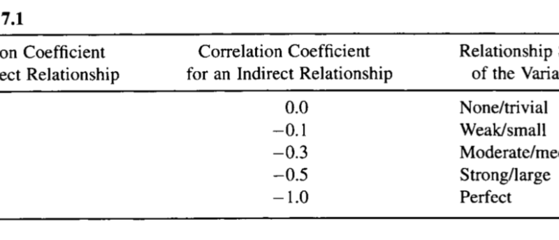
Correlation quantifies this association, often as a measure between the values -1 to 1 for perfectly negatively correlated and perfectly positively correlated. The calculated correlation is referred to as the “correlation coefficient.” This correlation coefficient can then be interpreted to describe the measures.
See the table below to help with interpretation the correlation coefficient.
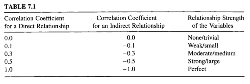
Table of Correlation Coefficient Values and Their Interpretation
Taken from “Nonparametric Statistics for Non-Statisticians: A Step-by-Step Approach”.
The correlation between two variables that each have a Gaussian distribution can be calculated using standard methods such as the Pearson’s correlation. This procedure cannot be used for data that does not have a Gaussian distribution. Instead, rank correlation methods must be used.
Rank correlation refers to methods that quantify the association between variables using the ordinal relationship between the values rather than the specific values. Ordinal data is data that has label values and has an order or rank relationship; for example: ‘low‘, ‘medium‘, and ‘high‘.
Rank correlation can be calculated for real-valued variables. This is done by first converting the values for each variable into rank data. This is where the values are ordered and assigned an integer rank value. Rank correlation coefficients can then be calculated in order to quantify the association between the two ranked variables.
Because no distribution for the values is assumed, rank correlation methods are referred to as distribution-free correlation or nonparametric correlation. Interestingly, rank correlation measures are often used as the basis for other statistical hypothesis tests, such as determining whether two samples were likely drawn from the same (or different) population distributions.
Rank correlation methods are often named after the researcher or researchers that developed the method. Four examples of rank correlation methods are as follows:
- Spearman’s Rank Correlation.
- Kendall’s Rank Correlation.
- Goodman and Kruskal’s Rank Correlation.
- Somers’ Rank Correlation.
In the following sections, we will take a closer look at two of the more common rank correlation methods: Spearman’s and Kendall’s.
Test Dataset
Before we demonstrate rank correlation methods, we must first define a test problem.
In this section, we will define a simple two-variable dataset where each variable is drawn from a uniform distribution (e.g. non-Gaussian) and the values of the second variable depend on the values of the first value.
Specifically, a sample of 1,000 random floating point values are drawn from a uniform distribution and scaled to the range 0 to 20. A second sample of 1,000 random floating point values are drawn from a uniform distribution between 0 and 10 and added to values in the first sample to create an association.
# prepare data
data1 = rand(1000) * 20
data2 = data1 + (rand(1000) * 10)
The complete example is listed below.
# generate related variables
from numpy.random import rand
from numpy.random import seed
from matplotlib import pyplot
# seed random number generator
seed(1)
# prepare data
data1 = rand(1000) * 20
data2 = data1 + (rand(1000) * 10)
# plot
pyplot.scatter(data1, data2)
pyplot.show()
Running the example generates the data sample and graphs the points on a scatter plot.
We can clearly see that each variable has a uniform distribution and the positive association between the variables is visible by the diagonal grouping of the points from the bottom left to the top right of the plot.
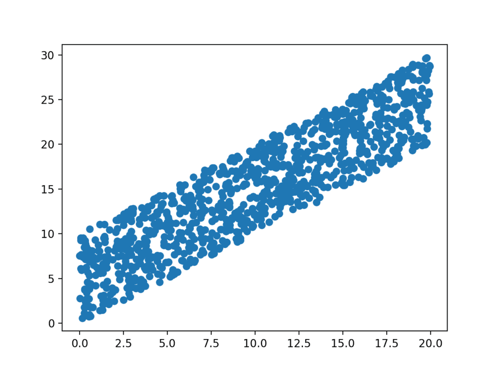
Scatter Plot of Associated Variables Drawn From a Uniform Distribution
Spearman’s Rank Correlation
Spearman’s rank correlation is named for Charles Spearman.
It may also be called Spearman’s correlation coefficient and is denoted by the lowercase greek letter rho (p). As such, it may be referred to as Spearman’s rho.
This statistical method quantifies the degree to which ranked variables are associated by a monotonic function, meaning an increasing or decreasing relationship. As a statistical hypothesis test, the method assumes that the samples are uncorrelated (fail to reject H0).
The Spearman rank-order correlation is a statistical procedure that is designed to measure the relationship between two variables on an ordinal scale of measurement.
— Page 124, Nonparametric Statistics for Non-Statisticians: A Step-by-Step Approach, 2009.
The intuition for the Spearman’s rank correlation is that it calculates a Pearson’s correlation (e.g. a parametric measure of correlation) using the rank values instead of the real values. Where the Pearson’s correlation is the calculation of the covariance (or expected difference of observations from the mean) between the two variables normalized by the variance or spread of both variables.
Spearman’s rank correlation can be calculated in Python using the spearmanr() SciPy function.
The function takes two real-valued samples as arguments and returns both the correlation coefficient in the range between -1 and 1 and the p-value for interpreting the significance of the coefficient.
# calculate spearman's correlation
coef, p = spearmanr(data1, data2)
We can demonstrate the Spearman’s rank correlation on the test dataset. We know that there is a strong association between the variables in the dataset and we would expect the Spearman’s test to find this association.
The complete example is listed below.
# calculate the spearman's correlation between two variables
from numpy.random import rand
from numpy.random import seed
from scipy.stats import spearmanr
# seed random number generator
seed(1)
# prepare data
data1 = rand(1000) * 20
data2 = data1 + (rand(1000) * 10)
# calculate spearman's correlation
coef, p = spearmanr(data1, data2)
print('Spearmans correlation coefficient: %.3f' % coef)
# interpret the significance
alpha = 0.05
if p > alpha:
	print('Samples are uncorrelated (fail to reject H0) p=%.3f' % p)
else:
	print('Samples are correlated (reject H0) p=%.3f' % p)
Running the example calculates the Spearman’s correlation coefficient between the two variables in the test dataset.
The statistical test reports a strong positive correlation with a value of 0.9. The p-value is close to zero, which means that the likelihood of observing the data given that the samples are uncorrelated is very unlikely (e.g. 95% confidence) and that we can reject the null hypothesis that the samples are uncorrelated.
Spearmans correlation coefficient: 0.900
Samples are correlated (reject H0) p=0.000
Kendall’s Rank Correlation
Kendall’s rank correlation is named for Maurice Kendall.
It is also called Kendall’s correlation coefficient, and the coefficient is often referred to by the lowercase Greek letter tau (t). In turn, the test may be called Kendall’s tau.
The intuition for the test is that it calculates a normalized score for the number of matching or concordant rankings between the two samples. As such, the test is also referred to as Kendall’s concordance test.
The Kendall’s rank correlation coefficient can be calculated in Python using the kendalltau() SciPy function. The test takes the two data samples as arguments and returns the correlation coefficient and the p-value. As a statistical hypothesis test, the method assumes (H0) that there is no association between the two samples.
# calculate kendall's correlation
coef, p = kendalltau(data1, data2)
We can demonstrate the calculation on the test dataset, where we do expect a significant positive association to be reported.
The complete example is listed below.
# calculate the kendall's correlation between two variables
from numpy.random import rand
from numpy.random import seed
from scipy.stats import kendalltau
# seed random number generator
seed(1)
# prepare data
data1 = rand(1000) * 20
data2 = data1 + (rand(1000) * 10)
# calculate kendall's correlation
coef, p = kendalltau(data1, data2)
print('Kendall correlation coefficient: %.3f' % coef)
# interpret the significance
alpha = 0.05
if p > alpha:
	print('Samples are uncorrelated (fail to reject H0) p=%.3f' % p)
else:
	print('Samples are correlated (reject H0) p=%.3f' % p)
Running the example calculates the Kendall’s correlation coefficient as 0.7, which is highly correlated.
The p-value is close to zero (and printed as zero), as with the Spearman’s test, meaning that we can confidently reject the null hypothesis that the samples are uncorrelated.
Kendall correlation coefficient: 0.709
Samples are correlated (reject H0) p=0.000
Extensions
This section lists some ideas for extending the tutorial that you may wish to explore.
- List three examples where calculating a nonparametric correlation coefficient might be useful during a machine learning project.
- Update each example to calculate the correlation between uncorrelated data samples drawn from a non-Gaussian distribution.
- Load a standard machine learning dataset and calculate the pairwise nonparametric correlation between all variables.
If you explore any of these extensions, I’d love to know.
Further Reading
This section provides more resources on the topic if you are looking to go deeper.
Books
- Nonparametric Statistics for Non-Statisticians: A Step-by-Step Approach, 2009.
- Applied Nonparametric Statistical Methods, Fourth Edition, 2007.
- Rank Correlation Methods, 1990.
API
Articles
- Nonparametric statistics on Wikipedia
- Rank correlation on Wikipedia
- Spearman’s rank correlation coefficient on Wikipedia
- Kendall rank correlation coefficient on Wikipedia
- Goodman and Kruskal’s gamma on Wikipedia
- Somers’ D on Wikipedia
Summary
In this tutorial, you discovered rank correlation methods for quantifying the association between variables with a non-Gaussian distribution.
Specifically, you learned:
- How rank correlation methods work and the methods are that are available.
- How to calculate and interpret the Spearman’s rank correlation coefficient in Python.
- How to calculate and interpret the Kendall’s rank correlation coefficient in Python.
Do you have any questions?
Ask your questions in the comments below and I will do my best to answer.
The post How to Calculate Nonparametric Rank Correlation in Python appeared first on Machine Learning Mastery.