Author: Jason Brownlee
A Case Study in How to Avoid Methodological Errors when
Evaluating Machine Learning Methods for Time Series Forecasting.
Evaluating machine learning models on time series forecasting problems is challenging.
It is easy to make a small error in the framing of a problem or in the evaluation of models that give impressive results but result in an invalid finding.
An interesting time series classification problem is predicting whether a subject’s eyes are open or closed based only on their brain wave data (EEG).
In this tutorial, you will discover the problem of predicting whether eyes are open or closed based on brain waves and a common methodological trap when evaluating time series forecasting models.
Working through this tutorial, you will have an idea of how to avoid common traps when evaluating machine learning algorithms on time series forecast problems. These are traps that catch both beginners, expert practitioners, and academics alike.
After completing this tutorial, you will know:
- The eye-state prediction problem and a standard machine learning dataset that you can use.
- How to reproduce skilful results for predicting eye-state from brainwaves in Python.
- How to uncover an interesting methodological flaw in evaluating forecast models.
Let’s get started.
Tutorial Overview
This tutorial is divided into seven parts; they are:
- Predict Open/Closed Eyes from Brain Waves
- Data Visualization and Remove Outliers
- Develop the Predictive Model
- Problem with the Model Evaluation Methodology
- Train-Test Split with Temporal Ordering
- Walk-Forward Validation
- Takeaways and Key Lesson
Predict Open/Closed Eyes from Brain Waves
In this post, we are going to take a closer look at a problem that involves predicting whether the subjects eyes are open or closed based on brain wave data.
The problem was described and data collected by Oliver Rosler and David Suendermann for their 2013 paper titled “A First Step towards Eye State Prediction Using EEG“.
I saw this dataset and I had to know more.
Specifically, an electroencephalography (EEG) recording was made of a single person for 117 seconds (just under two minutes) while the subject opened and closed their eyes, which was recorded via a video camera. The open/closed state was then recorded against each time step in the EEG trace manually.
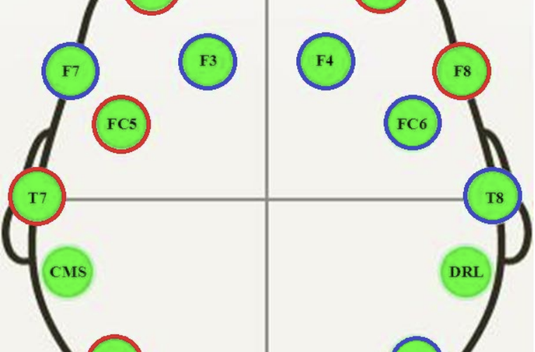
The EEG was recorded using a Emotiv EEG Neuroheadset, resulting in 14 traces.
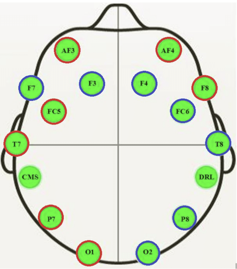
Cartoon of where EEG sensors were located on the subject
Taken from “A First Step towards Eye State Prediction Using EEG”, 2013.
The output variable is binary, meaning that this is a two-class classification problem.
A total of 14,980 observations (rows) were made over the 117 seconds, meaning that there were about 128 observations per second.
The corpus consists of 14,977 instances with 15 attributes each (14 attributes representing the values of the electrodes and the eye state). The instances are stored in the corpus in chronological order to be able to analyze temporal dependencies. 8,255 (55.12%) instances of the corpus correspond to the eye open and 6,722 (44.88%) instances to the eye closed state.
There were also some EEG observations that have a much larger than expected amplitude. These are likely outliers and can be identified and removed using a simple statistical method such as removing rows that have an observation 3-to-4 standard deviations from the mean.
The simplest framing of the problem is to predict the eye-state (open/closed) given the EEG trace at the current time step. More advanced framings of the problem may seek to model the multivariate time series of each EEG trace in order to predict the current eye state.
Data Visualization and Remove Outliers
The dataset can be downloaded for free from the UCI Machine Learning repository:
The raw data is in ARFF format (used in Weka), but can be converted to CSV by deleting the ARFF header.
Below is a sample of the first five lines of the data with the ARFF header removed.
4329.23,4009.23,4289.23,4148.21,4350.26,4586.15,4096.92,4641.03,4222.05,4238.46,4211.28,4280.51,4635.9,4393.85,0
4324.62,4004.62,4293.85,4148.72,4342.05,4586.67,4097.44,4638.97,4210.77,4226.67,4207.69,4279.49,4632.82,4384.1,0
4327.69,4006.67,4295.38,4156.41,4336.92,4583.59,4096.92,4630.26,4207.69,4222.05,4206.67,4282.05,4628.72,4389.23,0
4328.72,4011.79,4296.41,4155.9,4343.59,4582.56,4097.44,4630.77,4217.44,4235.38,4210.77,4287.69,4632.31,4396.41,0
4326.15,4011.79,4292.31,4151.28,4347.69,4586.67,4095.9,4627.69,4210.77,4244.1,4212.82,4288.21,4632.82,4398.46,0
...
We can load the data as a DataFrame and plot the time series for each EEG trace and the output variable (open/closed state).
The complete code example is listed below.
The example assumes that you have a copy of the dataset in CSV format with the filename ‘EEG_Eye_State.csv‘ in the same directory as the code.
# visualize dataset
from pandas import read_csv
from matplotlib import pyplot
# load the dataset
data = read_csv('EEG_Eye_State.csv', header=None)
# retrieve data as numpy array
values = data.values
# create a subplot for each time series
pyplot.figure()
for i in range(values.shape[1]):
	pyplot.subplot(values.shape[1], 1, i+1)
	pyplot.plot(values[:, i])
pyplot.show()
Running the example creates a line plot for each EEG trace and the output variable.
We can see the outliers washing out the data in each trace. We can also see the open/closed state of the eyes over time with 0/1 respectively.
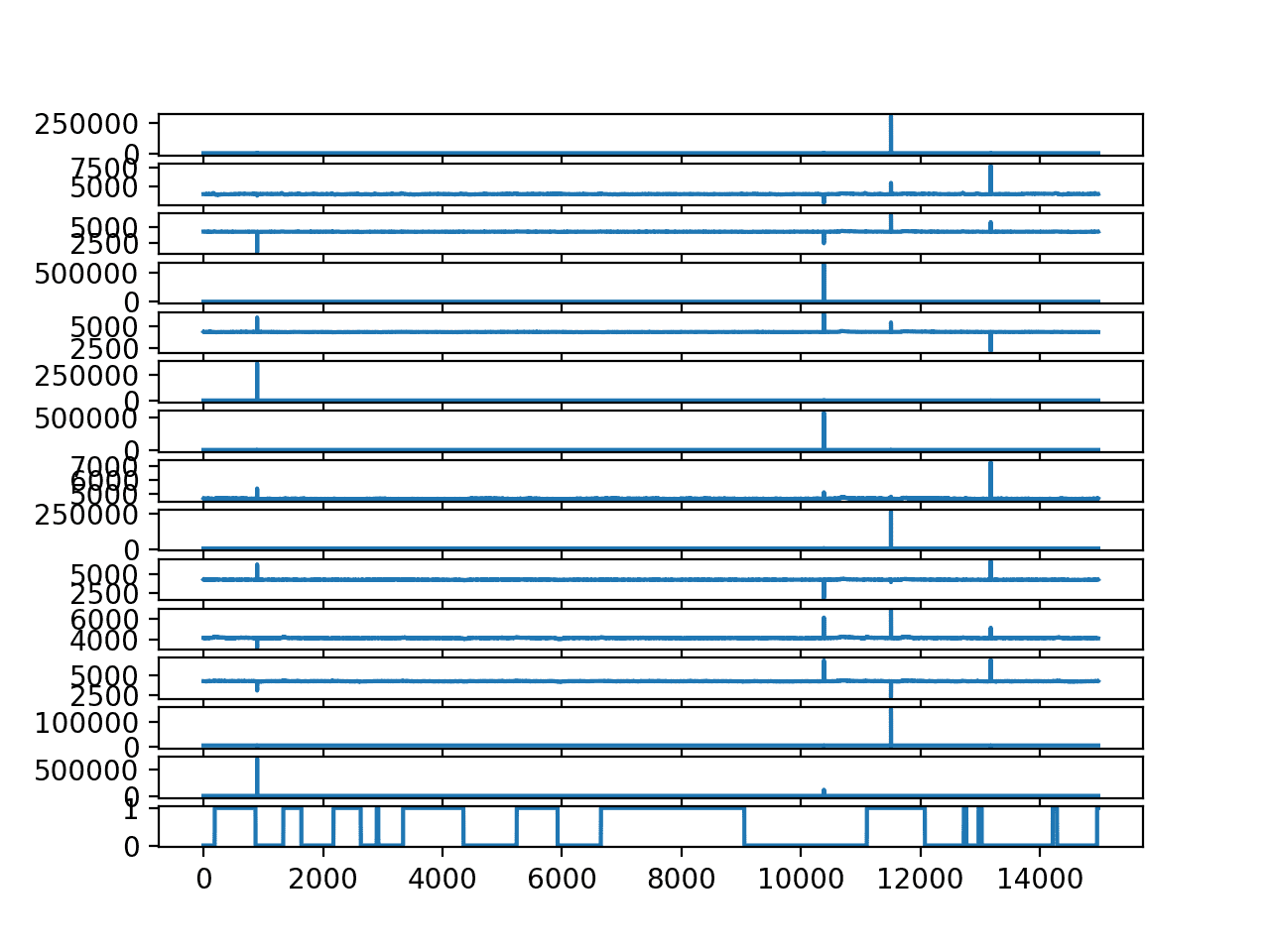
Line Plot for each EEG trace and the output variable
It is useful to remove the outliers to better understand the relationship between the EEG traces and the open/closed state of the eyes.
The example below removes all rows that have an EEG observation that is four standard deviations or more from the mean. The dataset is saved to a new file called ‘EEG_Eye_State_no_outliers.csv‘.
It is a quick and dirty implementation of outlier detection and removal, but gets the job done. I’m sure you could engineer a more efficient implementation.
# remove outliers from the EEG data
from pandas import read_csv
from numpy import mean
from numpy import std
from numpy import delete
from numpy import savetxt
# load the dataset.
data = read_csv('EEG_Eye_State.csv', header=None)
values = data.values
# step over each EEG column
for i in range(values.shape[1] - 1):
	# calculate column mean and standard deviation
	data_mean, data_std = mean(values[:,i]), std(values[:,i])
	# define outlier bounds
	cut_off = data_std * 4
	lower, upper = data_mean - cut_off, data_mean + cut_off
	# remove too small
	too_small = [j for j in range(values.shape[0]) if values[j,i] < lower]
	values = delete(values, too_small, 0)
	print('>deleted %d rows' % len(too_small))
	# remove too large
	too_large = [j for j in range(values.shape[0]) if values[j,i] > upper]
	values = delete(values, too_large, 0)
	print('>deleted %d rows' % len(too_large))
# save the results to a new file
savetxt('EEG_Eye_State_no_outliers.csv', values, delimiter=',')
Running the example summarizes the rows deleted as each column in the EEG data is processed for outliers above and below the mean.
>deleted 0 rows
>deleted 1 rows
>deleted 2 rows
>deleted 1 rows
>deleted 0 rows
>deleted 142 rows
>deleted 0 rows
>deleted 48 rows
>deleted 0 rows
>deleted 153 rows
>deleted 0 rows
>deleted 43 rows
>deleted 0 rows
>deleted 0 rows
>deleted 0 rows
>deleted 15 rows
>deleted 0 rows
>deleted 5 rows
>deleted 10 rows
>deleted 0 rows
>deleted 21 rows
>deleted 53 rows
>deleted 0 rows
>deleted 12 rows
>deleted 58 rows
>deleted 53 rows
>deleted 0 rows
>deleted 59 rows
We can now visualize the data without outliers by loading the new ‘EEG_Eye_State_no_outliers.csv‘ file.
# visualize dataset without outliers
from pandas import read_csv
from matplotlib import pyplot
# load the dataset
data = read_csv('EEG_Eye_State_no_outliers.csv', header=None)
# retrieve data as numpy array
values = data.values
# create a subplot for each time series
pyplot.figure()
for i in range(values.shape[1]):
	pyplot.subplot(values.shape[1], 1, i+1)
	pyplot.plot(values[:, i])
pyplot.show()
Running the example creates a better plot, clearly showing little positive peaks when eyes are closed (1) and negative peaks when eyes are open (0).
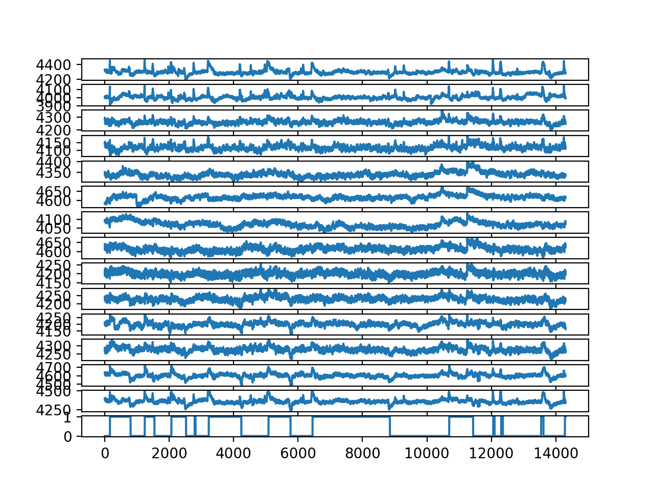
Line Plot for each EEG trace and the output variable without outliers
Develop the Predictive Model
The simplest predictive model is to predict the eye open/closed state based on the current EEG observation, ignoring the trace information.
Intuitively, one would not expect this to be effective, nevertheless, it was the approach used in Rosler and Suendermann’s 2013 paper.
Specifically, they evaluated a large suite of classification algorithms in the Weka software using 10-fold cross-validation of this framing of the problem. They achieved better than 90% accuracy with multiple methods, including instance based methods such as k-nearest neighbors and KStar.
However, instance-based learners such as IB1 and KStar outperformed decision trees yet again substantially. The latter achieved the clearly best performance with a classification error rate of merely 3.2%.
— A First Step towards Eye State Prediction Using EEG, 2013.
A similar methodology and finding was used with the same and similar datasets in a number of other papers.
I was surprised when I read this and so reproduced the result.
The complete example is listed below with a k=3 KNN.
# knn for predicting eye state
from pandas import read_csv
from sklearn.metrics import accuracy_score
from sklearn.model_selection import KFold
from sklearn.neighbors import KNeighborsClassifier
from numpy import mean
# load the dataset
data = read_csv('EEG_Eye_State_no_outliers.csv', header=None)
values = data.values
# evaluate knn using 10-fold cross-validation
scores = list()
kfold = KFold(10, shuffle=True, random_state=1)
for train_ix, test_ix in kfold.split(values):
	# define train/test X/y
	trainX, trainy = values[train_ix, :-1], values[train_ix, -1]
	testX, testy = values[test_ix, :-1], values[test_ix, -1]
	# define model
	model = KNeighborsClassifier(n_neighbors=3)
	# fit model on train set
	model.fit(trainX, trainy)
	# forecast test set
	yhat = model.predict(testX)
	# evaluate predictions
	score = accuracy_score(testy, yhat)
	# store
	scores.append(score)
	print('>%.3f' % score)
# calculate mean score across each run
print('Final Score: %.3f' % (mean(scores)))
Running the example prints the score for each fold of the cross validation and the mean score of 97% averaged across all 10 folds.
>0.970
>0.975
>0.978
>0.977
>0.973
>0.979
>0.978
>0.976
>0.974
>0.969
Final Score: 0.975
Very impressive!
But something felt wrong.
I was interested to see how models that took into account the clear peaks in the data at each transition from open-to-closed and closed-to-open performed.
Every model I tried using my own test harness that respected the temporal ordering of the data performed much worse.
Why?
Hint: think about the chosen model evaluation strategy and the type of algorithm that performed the best.
Problem with the Model Evaluation Methodology
Disclaimer: I am not calling out the authors of the paper or related papers. I don’t care. In my experience, most published papers cannot be reproduced or have major methodological flaws (including a lot of the stuff that I have written). I’m only interested in learning and teaching.
There is a methodological flaw in the way that time series models are evaluated.
I coach against this flaw, but after reading the paper and reproducing the result, it still tripped me up.
I hope by working through this example that it will help not trip you up on your own forecast problems.
The methodological flaw in the evaluation of the models is the use of k-fold cross-validation. Specifically, the evaluation of the models in a way that does not respect the temporal ordering of the observations.
Key to this problem is the finding of instance-based methods, such as k-nearest neighbors, as being skillful on the problem. KNN will seek out the k most similar rows in the dataset and calculate the mode of the output state as the prediction.
By not respecting the temporal order of instances when evaluating models, it allows the models to use information from the future in making the prediction. This is pronounced specifically in the KNN algorithm.
Because of the high frequency of observations (128 per second), the most similar rows will be those adjacent in time to the instance being predicted, both in the past and in the future.
We can make this clearer with some small experiments.
Train-Test Split with Temporal Ordering
The first test we can do is to evaluate the skill of a KNN model with a train/test split both when the dataset is shuffled, and when it is not.
In the case when the data is shuffled prior to the split, we expect the result to be similar to the cross-validation result in the previous section, specifically if the test set is 10% of the dataset.
If the theory about the importance of temporal ordering and instance-based methods using adjacent examples in the future is true, we would expect the test where the dataset is not shuffled prior to the split to be worse.
First, the example below splits the dataset into train/test split with 90%/10% of the data respectively. The dataset is shuffled prior to the split.
# knn for predicting eye state
from pandas import read_csv
from sklearn.metrics import accuracy_score
from sklearn.model_selection import train_test_split
from sklearn.neighbors import KNeighborsClassifier
# load the dataset
data = read_csv('EEG_Eye_State_no_outliers.csv', header=None)
values = data.values
# split data into inputs and outputs
X, y = values[:, :-1], values[:, -1]
# split the dataset
trainX, testX, trainy, testy = train_test_split(X, y, test_size=0.1, shuffle=True, random_state=1)
# define model
model = KNeighborsClassifier(n_neighbors=3)
# fit model on train set
model.fit(trainX, trainy)
# forecast test set
yhat = model.predict(testX)
# evaluate predictions
score = accuracy_score(testy, yhat)
print(score)
Running the example, we can see that indeed, the skill matches what we see in the cross-validation example, or close to it, at 96% accuracy.
0.9699510831586303
Next, we repeat the experiment without shuffling the dataset prior to the split.
This means that the training data are the first 90% of the data respecting the temporal ordering of the observations, and the test dataset is the last 10%, or about 1,400 observations of the data.
# knn for predicting eye state
from pandas import read_csv
from sklearn.metrics import accuracy_score
from sklearn.model_selection import train_test_split
from sklearn.neighbors import KNeighborsClassifier
# load the dataset
data = read_csv('EEG_Eye_State_no_outliers.csv', header=None)
values = data.values
# split data into inputs and outputs
X, y = values[:, :-1], values[:, -1]
# split the dataset
trainX, testX, trainy, testy = train_test_split(X, y, test_size=0.1, shuffle=False, random_state=1)
# define model
model = KNeighborsClassifier(n_neighbors=3)
# fit model on train set
model.fit(trainX, trainy)
# forecast test set
yhat = model.predict(testX)
# evaluate predictions
score = accuracy_score(testy, yhat)
print(score)
Running the example shows model skill that is much worse at 52%.
0.5269042627533194
This is a good start, but not definitive.
It is possible that the last 10% of the dataset is hard to predict, given the very short open/close intervals we can see on the plot of the outcome variable.
We can repeat the experiment and use the first 10% of the data in time for test and the last 90% for train. We can do this by reversing the order of the rows prior to splitting the data using the flip() function.
# knn for predicting eye state
from pandas import read_csv
from sklearn.metrics import accuracy_score
from sklearn.model_selection import train_test_split
from sklearn.neighbors import KNeighborsClassifier
from numpy import flip
# load the dataset
data = read_csv('EEG_Eye_State_no_outliers.csv', header=None)
values = data.values
# reverse order of rows
values = flip(values, 0)
# split data into inputs and outputs
X, y = values[:, :-1], values[:, -1]
# split the dataset
trainX, testX, trainy, testy = train_test_split(X, y, test_size=0.1, shuffle=False, random_state=1)
# define model
model = KNeighborsClassifier(n_neighbors=3)
# fit model on train set
model.fit(trainX, trainy)
# forecast test set
yhat = model.predict(testX)
# evaluate predictions
score = accuracy_score(testy, yhat)
print(score)
Running the experiment produces similar results at about 52% accuracy.
This gives more evidence that it is not the specific contiguous block of observations that results in the poor model skill.
0.5290006988120196
It looks like immediately adjacent observations are required to make good predictions.
Walk-Forward Validation
It is possible that the model requires the adjacent observations in the past (but not the future) in order to make skillful predictions.
This sounds reasonable at first, but also has a problem.
Nevertheless we can achieve this using walk-forward validation over the test set. This is where the model is permitted to use all observations prior to the time step being predicted as we validate a new model at each new time step in the test dataset.
For more on walk-forward validation, see the post:
The example below evaluates the skill of KNN using walk-forward validation over the last 10% of the dataset (about 10 seconds), respecting temporal ordering.
# knn for predicting eye state
from pandas import read_csv
from sklearn.metrics import accuracy_score
from sklearn.model_selection import train_test_split
from sklearn.neighbors import KNeighborsClassifier
from numpy import array
# load the dataset
data = read_csv('EEG_Eye_State_no_outliers.csv', header=None)
values = data.values
# split data into inputs and outputs
X, y = values[:, :-1], values[:, -1]
# split the dataset
trainX, testX, trainy, testy = train_test_split(X, y, test_size=0.1, shuffle=False, random_state=1)
# walk-forward validation
historyX, historyy = [x for x in trainX], [x for x in trainy]
predictions = list()
for i in range(len(testy)):
	# define model
	model = KNeighborsClassifier(n_neighbors=3)
	# fit model on train set
	model.fit(array(historyX), array(historyy))
	# forecast the next time step
	yhat = model.predict([testX[i, :]])[0]
	# store prediction
	predictions.append(yhat)
	# add real observation to history
	historyX.append(testX[i, :])
	historyy.append(testy[i])
# evaluate predictions
score = accuracy_score(testy, predictions)
print(score)
Running the example gives an impressive model skill at about 95% accuracy.
0.9531795946890287
We can push this test further and only make the previous 10 observations available to the model when making a prediction.
The complete example is listed below.
# knn for predicting eye state
from pandas import read_csv
from sklearn.metrics import accuracy_score
from sklearn.model_selection import train_test_split
from sklearn.neighbors import KNeighborsClassifier
from numpy import array
# load the dataset
data = read_csv('EEG_Eye_State_no_outliers.csv', header=None)
values = data.values
# split data into inputs and outputs
X, y = values[:, :-1], values[:, -1]
# split the dataset
trainX, testX, trainy, testy = train_test_split(X, y, test_size=0.1, shuffle=False, random_state=1)
# walk-forward validation
historyX, historyy = [x for x in trainX], [x for x in trainy]
predictions = list()
for i in range(len(testy)):
	# define model
	model = KNeighborsClassifier(n_neighbors=3)
	# fit model on a small subset of the train set
	tmpX, tmpy = array(historyX)[-10:,:], array(historyy)[-10:]
	model.fit(tmpX, tmpy)
	# forecast the next time step
	yhat = model.predict([testX[i, :]])[0]
	# store prediction
	predictions.append(yhat)
	# add real observation to history
	historyX.append(testX[i, :])
	historyy.append(testy[i])
# evaluate predictions
score = accuracy_score(testy, predictions)
print(score)
Running the example results in a further improved model skill of nearly 99% accuracy.
I would expect that the only errors being made are those at the inflection points in the EEG series when the trace transitions from open-to-closed or closed-to-open, the actual hard part of the problem. This aspect requires further investigation.
0.9923130677847659
Indeed, we have confirmed that the model requires adjacent observations and their outcome in order to make a prediction, and that it can do very well with only adjacent observations in the past, not the future.
This is interesting. But this finding is not useful in practice.
If this model was deployed, it would require the model to know the eye open/closed state in the very recent past, such as the previous 128th of a second.
This will not be available.
The whole idea of a model for predicting eye state based on brain waves is to have it operate without such confirmation.
Takeaways and Key Lesson
Let’s review what we have learned so far:
1. The model evaluation methodology must take the temporal ordering of observations into account.
This means that it is methodologically invalid to use k-fold cross-validation that does not stratify by time (e.g. shuffles or uses a random selection of rows).
This also means that it is methodologically invalid to use a train/test split that shuffles the data prior to splitting.
We saw this in the evaluation of the high skill of the model with k-fold cross-validation and shuffled train/test split compared to the low skill of the model when directly adjacent observations in time were not available at prediction time.
2. The model evaluation methodology must make sense for the use of the final model.
This means that even if you use a methodology that respects the temporal ordering of the observations, the model should only have information available that it would have if the model were being used in practice.
We saw this in the high skill of the model under a walk-forward validation methodology that respected the order of observations, but made information available, such as eye-state, that would not be available if the model were being used in practice.
The key is to start with a framing of the problem based in the use of the final model and work backwards to the data that would be available and a methodology for evaluating the model in its framing that only operates under information that would be available in that framing.
This applies doubly when you are trying to understand other people’s work.
Going Forward
Hopefully, this helps, both when you are evaluating your own forecast models and when you are evaluating the models of others.
So, how would you work this problem if presented with the raw data?
I think the keys to this problem are the positive/negative peaks that are obvious in the EEG data at the times when there is a transition from eyes open-to-closed or closed-to-open. I would expect an effective model would exploit this feature, perhaps using half a second or similar of prior EEG observations.
This might even be possible with a single trace, rather than 15, and a simple peak detection method from signal processing, rather than a machine learning method.
Let me know if you have a go at this; I’d love to see what you discover.
Further Reading
This section provides more resources on the topic if you are looking to go deeper.
- EEG Eye State Data Set, UCI Machine Learning Repository
- A First Step towards Eye State Prediction Using EEG, 2013.
- EEG Eye State Identification Using Incremental Attribute Learning with Time-Series Classification, 2014.
Summary
In this tutorial, you discovered the problem of predicting whether eyes are open or closed based on brain waves and a common methodological trap when evaluating time series forecasting models.
Specifically, you learned:
- The eye-state prediction problem and a standard machine learning dataset that you can use.
- How to reproduce skilful results for predicting eye-state from brainwaves in Python.
- How to uncover an interesting methodological flaw in evaluating forecast models.
Do you have any questions?
Ask your questions in the comments below and I will do my best to answer.
The post How to Predict Whether a Persons Eyes are Open or Closed Using Brain Waves appeared first on Machine Learning Mastery.