
Author: Jason Brownlee
Given the rise of smart electricity meters and the wide adoption of electricity generation technology like solar panels, there is a wealth of electricity usage data available.
This data represents a multivariate time series of power-related variables that in turn could be used to model and even forecast future electricity consumption.
Machine learning algorithms predict a single value and cannot be used directly for multi-step forecasting. Two strategies that can be used to make multi-step forecasts with machine learning algorithms are the recursive and the direct methods.
In this tutorial, you will discover how to develop recursive and direct multi-step forecasting models with machine learning algorithms.
After completing this tutorial, you will know:
- How to develop a framework for evaluating linear, nonlinear, and ensemble machine learning algorithms for multi-step time series forecasting.
- How to evaluate machine learning algorithms using a recursive multi-step time series forecasting strategy.
- How to evaluate machine learning algorithms using a direct per-day and per-lead time multi-step time series forecasting strategy.
Let’s get started.

Multi-step Time Series Forecasting with Machine Learning Models for Household Electricity Consumption
Photo by Sean McMenemy, some rights reserved.
Tutorial Overview
This tutorial is divided into five parts; they are:
- Problem Description
- Load and Prepare Dataset
- Model Evaluation
- Recursive Multi-Step Forecasting
- Direct Multi-Step Forecasting
Problem Description
The ‘Household Power Consumption‘ dataset is a multivariate time series dataset that describes the electricity consumption for a single household over four years.
The data was collected between December 2006 and November 2010 and observations of power consumption within the household were collected every minute.
It is a multivariate series comprised of seven variables (besides the date and time); they are:
- global_active_power: The total active power consumed by the household (kilowatts).
- global_reactive_power: The total reactive power consumed by the household (kilowatts).
- voltage: Average voltage (volts).
- global_intensity: Average current intensity (amps).
- sub_metering_1: Active energy for kitchen (watt-hours of active energy).
- sub_metering_2: Active energy for laundry (watt-hours of active energy).
- sub_metering_3: Active energy for climate control systems (watt-hours of active energy).
Active and reactive energy refer to the technical details of alternative current.
A fourth sub-metering variable can be created by subtracting the sum of three defined sub-metering variables from the total active energy as follows:
sub_metering_remainder = (global_active_power * 1000 / 60) - (sub_metering_1 + sub_metering_2 + sub_metering_3)
Load and Prepare Dataset
The dataset can be downloaded from the UCI Machine Learning repository as a single 20 megabyte .zip file:
Download the dataset and unzip it into your current working directory. You will now have the file “household_power_consumption.txt” that is about 127 megabytes in size and contains all of the observations.
We can use the read_csv() function to load the data and combine the first two columns into a single date-time column that we can use as an index.
# load all data
dataset = read_csv('household_power_consumption.txt', sep=';', header=0, low_memory=False, infer_datetime_format=True, parse_dates={'datetime':[0,1]}, index_col=['datetime'])
Next, we can mark all missing values indicated with a ‘?‘ character with a NaN value, which is a float.
This will allow us to work with the data as one array of floating point values rather than mixed types (less efficient.)
# mark all missing values
dataset.replace('?', nan, inplace=True)
# make dataset numeric
dataset = dataset.astype('float32')
We also need to fill in the missing values now that they have been marked.
A very simple approach would be to copy the observation from the same time the day before. We can implement this in a function named fill_missing() that will take the NumPy array of the data and copy values from exactly 24 hours ago.
# fill missing values with a value at the same time one day ago
def fill_missing(values):
	one_day = 60 * 24
	for row in range(values.shape[0]):
		for col in range(values.shape[1]):
			if isnan(values[row, col]):
				values[row, col] = values[row - one_day, col]
We can apply this function directly to the data within the DataFrame.
# fill missing
fill_missing(dataset.values)
Now we can create a new column that contains the remainder of the sub-metering, using the calculation from the previous section.
# add a column for for the remainder of sub metering
values = dataset.values
dataset['sub_metering_4'] = (values[:,0] * 1000 / 60) - (values[:,4] + values[:,5] + values[:,6])
We can now save the cleaned-up version of the dataset to a new file; in this case we will just change the file extension to .csv and save the dataset as ‘household_power_consumption.csv‘.
# save updated dataset
dataset.to_csv('household_power_consumption.csv')
Tying all of this together, the complete example of loading, cleaning-up, and saving the dataset is listed below.
# load and clean-up data
from numpy import nan
from numpy import isnan
from pandas import read_csv
from pandas import to_numeric

# fill missing values with a value at the same time one day ago
def fill_missing(values):
	one_day = 60 * 24
	for row in range(values.shape[0]):
		for col in range(values.shape[1]):
			if isnan(values[row, col]):
				values[row, col] = values[row - one_day, col]

# load all data
dataset = read_csv('household_power_consumption.txt', sep=';', header=0, low_memory=False, infer_datetime_format=True, parse_dates={'datetime':[0,1]}, index_col=['datetime'])
# mark all missing values
dataset.replace('?', nan, inplace=True)
# make dataset numeric
dataset = dataset.astype('float32')
# fill missing
fill_missing(dataset.values)
# add a column for for the remainder of sub metering
values = dataset.values
dataset['sub_metering_4'] = (values[:,0] * 1000 / 60) - (values[:,4] + values[:,5] + values[:,6])
# save updated dataset
dataset.to_csv('household_power_consumption.csv')
Running the example creates the new file ‘household_power_consumption.csv‘ that we can use as the starting point for our modeling project.
Need help with Deep Learning for Time Series?
Take my free 7-day email crash course now (with sample code).
Click to sign-up and also get a free PDF Ebook version of the course.
Model Evaluation
In this section, we will consider how we can develop and evaluate predictive models for the household power dataset.
This section is divided into four parts; they are:
- Problem Framing
- Evaluation Metric
- Train and Test Sets
- Walk-Forward Validation
Problem Framing
There are many ways to harness and explore the household power consumption dataset.
In this tutorial, we will use the data to explore a very specific question; that is:
Given recent power consumption, what is the expected power consumption for the week ahead?
This requires that a predictive model forecast the total active power for each day over the next seven days.
Technically, this framing of the problem is referred to as a multi-step time series forecasting problem, given the multiple forecast steps. A model that makes use of multiple input variables may be referred to as a multivariate multi-step time series forecasting model.
A model of this type could be helpful within the household in planning expenditures. It could also be helpful on the supply side for planning electricity demand for a specific household.
This framing of the dataset also suggests that it would be useful to downsample the per-minute observations of power consumption to daily totals. This is not required, but makes sense, given that we are interested in total power per day.
We can achieve this easily using the resample() function on the pandas DataFrame. Calling this function with the argument ‘D‘ allows the loaded data indexed by date-time to be grouped by day (see all offset aliases). We can then calculate the sum of all observations for each day and create a new dataset of daily power consumption data for each of the eight variables.
The complete example is listed below.
# resample minute data to total for each day
from pandas import read_csv
# load the new file
dataset = read_csv('household_power_consumption.csv', header=0, infer_datetime_format=True, parse_dates=['datetime'], index_col=['datetime'])
# resample data to daily
daily_groups = dataset.resample('D')
daily_data = daily_groups.sum()
# summarize
print(daily_data.shape)
print(daily_data.head())
# save
daily_data.to_csv('household_power_consumption_days.csv')
Running the example creates a new daily total power consumption dataset and saves the result into a separate file named ‘household_power_consumption_days.csv‘.
We can use this as the dataset for fitting and evaluating predictive models for the chosen framing of the problem.
Evaluation Metric
A forecast will be comprised of seven values, one for each day of the week ahead.
It is common with multi-step forecasting problems to evaluate each forecasted time step separately. This is helpful for a few reasons:
- To comment on the skill at a specific lead time (e.g. +1 day vs +3 days).
- To contrast models based on their skills at different lead times (e.g. models good at +1 day vs models good at days +5).
The units of the total power are kilowatts and it would be useful to have an error metric that was also in the same units. Both Root Mean Squared Error (RMSE) and Mean Absolute Error (MAE) fit this bill, although RMSE is more commonly used and will be adopted in this tutorial. Unlike MAE, RMSE is more punishing of forecast errors.
The performance metric for this problem will be the RMSE for each lead time from day 1 to day 7.
As a short-cut, it may be useful to summarize the performance of a model using a single score in order to aide in model selection.
One possible score that could be used would be the RMSE across all forecast days.
The function evaluate_forecasts() below will implement this behavior and return the performance of a model based on multiple seven-day forecasts.
# evaluate one or more weekly forecasts against expected values
def evaluate_forecasts(actual, predicted):
	scores = list()
	# calculate an RMSE score for each day
	for i in range(actual.shape[1]):
		# calculate mse
		mse = mean_squared_error(actual[:, i], predicted[:, i])
		# calculate rmse
		rmse = sqrt(mse)
		# store
		scores.append(rmse)
	# calculate overall RMSE
	s = 0
	for row in range(actual.shape[0]):
		for col in range(actual.shape[1]):
			s += (actual[row, col] - predicted[row, col])**2
	score = sqrt(s / (actual.shape[0] * actual.shape[1]))
	return score, scores
Running the function will first return the overall RMSE regardless of day, then an array of RMSE scores for each day.
Train and Test Sets
We will use the first three years of data for training predictive models and the final year for evaluating models.
The data in a given dataset will be divided into standard weeks. These are weeks that begin on a Sunday and end on a Saturday.
This is a realistic and useful way for using the chosen framing of the model, where the power consumption for the week ahead can be predicted. It is also helpful with modeling, where models can be used to predict a specific day (e.g. Wednesday) or the entire sequence.
We will split the data into standard weeks, working backwards from the test dataset.
The final year of the data is in 2010 and the first Sunday for 2010 was January 3rd. The data ends in mid November 2010 and the closest final Saturday in the data is November 20th. This gives 46 weeks of test data.
The first and last rows of daily data for the test dataset are provided below for confirmation.
2010-01-03,2083.4539999999984,191.61000000000055,350992.12000000034,8703.600000000033,3842.0,4920.0,10074.0,15888.233355799992
...
2010-11-20,2197.006000000004,153.76800000000028,346475.9999999998,9320.20000000002,4367.0,2947.0,11433.0,17869.76663959999
The daily data starts in late 2006.
The first Sunday in the dataset is December 17th, which is the second row of data.
Organizing the data into standard weeks gives 159 full standard weeks for training a predictive model.
2006-12-17,3390.46,226.0059999999994,345725.32000000024,14398.59999999998,2033.0,4187.0,13341.0,36946.66673200004
...
2010-01-02,1309.2679999999998,199.54600000000016,352332.8399999997,5489.7999999999865,801.0,298.0,6425.0,14297.133406600002
The function split_dataset() below splits the daily data into train and test sets and organizes each into standard weeks.
Specific row offsets are used to split the data using knowledge of the dataset. The split datasets are then organized into weekly data using the NumPy split() function.
# split a univariate dataset into train/test sets
def split_dataset(data):
	# split into standard weeks
	train, test = data[1:-328], data[-328:-6]
	# restructure into windows of weekly data
	train = array(split(train, len(train)/7))
	test = array(split(test, len(test)/7))
	return train, test
We can test this function out by loading the daily dataset and printing the first and last rows of data from both the train and test sets to confirm they match the expectations above.
The complete code example is listed below.
# split into standard weeks
from numpy import split
from numpy import array
from pandas import read_csv

# split a univariate dataset into train/test sets
def split_dataset(data):
	# split into standard weeks
	train, test = data[1:-328], data[-328:-6]
	# restructure into windows of weekly data
	train = array(split(train, len(train)/7))
	test = array(split(test, len(test)/7))
	return train, test

# load the new file
dataset = read_csv('household_power_consumption_days.csv', header=0, infer_datetime_format=True, parse_dates=['datetime'], index_col=['datetime'])
train, test = split_dataset(dataset.values)
# validate train data
print(train.shape)
print(train[0, 0, 0], train[-1, -1, 0])
# validate test
print(test.shape)
print(test[0, 0, 0], test[-1, -1, 0])
Running the example shows that indeed the train dataset has 159 weeks of data, whereas the test dataset has 46 weeks.
We can see that the total active power for the train and test dataset for the first and last rows match the data for the specific dates that we defined as the bounds on the standard weeks for each set.
(159, 7, 8)
3390.46 1309.2679999999998
(46, 7, 8)
2083.4539999999984 2197.006000000004
Walk-Forward Validation
Models will be evaluated using a scheme called walk-forward validation.
This is where a model is required to make a one week prediction, then the actual data for that week is made available to the model so that it can be used as the basis for making a prediction on the subsequent week. This is both realistic for how the model may be used in practice and beneficial to the models, allowing them to make use of the best available data.
We can demonstrate this below with separation of input data and output/predicted data.
Input, 						Predict
[Week1]						Week2
[Week1 + Week2]				Week3
[Week1 + Week2 + Week3]		Week4
...
The walk-forward validation approach to evaluating predictive models on this dataset is provided in a function below, named evaluate_model().
A scikit-learn model object is provided as an argument to the function, along with the train and test datasets. An additional argument n_input is provided that is used to define the number of prior observations that the model will use as input in order to make a prediction.
The specifics of how a scikit-learn model is fit and makes predictions is covered in later sections.
The forecasts made by the model are then evaluated against the test dataset using the previously defined evaluate_forecasts() function.
# evaluate a single model
def evaluate_model(model, train, test, n_input):
	# history is a list of weekly data
	history = [x for x in train]
	# walk-forward validation over each week
	predictions = list()
	for i in range(len(test)):
		# predict the week
		yhat_sequence = ...
		# store the predictions
		predictions.append(yhat_sequence)
		# get real observation and add to history for predicting the next week
		history.append(test[i, :])
	predictions = array(predictions)
	# evaluate predictions days for each week
	score, scores = evaluate_forecasts(test[:, :, 0], predictions)
	return score, scores
Once we have the evaluation for a model we can summarize the performance.
The function below, named summarize_scores(), will display the performance of a model as a single line for easy comparison with other models.
# summarize scores
def summarize_scores(name, score, scores):
	s_scores = ', '.join(['%.1f' % s for s in scores])
	print('%s: [%.3f] %s' % (name, score, s_scores))
We now have all of the elements to begin evaluating predictive models on the dataset.
Recursive Multi-Step Forecasting
Most predictive modeling algorithms will take some number of observations as input and predict a single output value.
As such, they cannot be used directly to make a multi-step time series forecast.
This applies to most linear, nonlinear, and ensemble machine learning algorithms.
One approach where machine learning algorithms can be used to make a multi-step time series forecast is to use them recursively.
This involves making a prediction for one time step, taking the prediction, and feeding it into the model as an input in order to predict the subsequent time step. This process is repeated until the desired number of steps have been forecasted.
For example:
X = [x1, x2, x3]
y1 = model.predict(X)

X = [x2, x3, y1]
y2 = model.predict(X)

X = [x3, y1, y2]
y3 = model.predict(X)

...
In this section, we will develop a test harness for fitting and evaluating machine learning algorithms provided in scikit-learn using a recursive model for multi-step forecasting.
The first step is to convert the prepared training data in window format into a single univariate series.
The to_series() function below will convert a list of weekly multivariate data into a single univariate series of daily total power consumed.
# convert windows of weekly multivariate data into a series of total power
def to_series(data):
	# extract just the total power from each week
	series = [week[:, 0] for week in data]
	# flatten into a single series
	series = array(series).flatten()
	return series
Next, the sequence of daily power needs to be transformed into inputs and outputs suitable for fitting a supervised learning problem.
The prediction will be some function of the total power consumed on prior days. We can choose the number of prior days to use as inputs, such as one or two weeks. There will always be a single output: the total power consumed on the next day.
The model will be fit on the true observations from prior time steps. We need to iterate through the sequence of daily power consumed and split it into inputs and outputs. This is called a sliding window data representation.
The to_supervised() function below implements this behavior.
It takes a list of weekly data as input as well as the number of prior days to use as inputs for each sample that is created.
The first step is to convert the history into a single data series. The series is then enumerated, creating one input and output pair per time step. This framing of the problem will allow a model to learn to predict any day of the week given the observations of prior days. The function returns the inputs (X) and outputs (y) ready for training a model.
# convert history into inputs and outputs
def to_supervised(history, n_input):
	# convert history to a univariate series
	data = to_series(history)
	X, y = list(), list()
	ix_start = 0
	# step over the entire history one time step at a time
	for i in range(len(data)):
		# define the end of the input sequence
		ix_end = ix_start + n_input
		# ensure we have enough data for this instance
		if ix_end < len(data):
			X.append(data[ix_start:ix_end])
			y.append(data[ix_end])
		# move along one time step
		ix_start += 1
	return array(X), array(y)
The scikit-learn library allows a model to be used as part of a pipeline. This allows data transforms to be applied automatically prior to fitting the model. More importantly, the transforms are prepared in the correct way, where they are prepared or fit on the training data and applied on the test data. This prevents data leakage when evaluating models.
We can use this capability when in evaluating models by creating a pipeline prior to fitting each model on the training dataset. We will both standardize and normalize the data prior to using the model.
The make_pipeline() function below implements this behavior, returning a Pipeline that can be used just like a model, e.g. it can be fit and it can make predictions.
The standardization and normalization operations are performed per column. In the to_supervised() function, we have essentially split one column of data (total power) into multiple columns, e.g. seven for seven days of input observations. This means that each of the seven columns in the input data will have a different mean and standard deviation for standardization and a different min and max for normalization.
Given that we used a sliding window, almost all values will appear in each column, therefore, this is not likely an issue. But it is important to note that it would be more rigorous to scale the data as a single column prior to splitting it into inputs and outputs.
# create a feature preparation pipeline for a model
def make_pipeline(model):
	steps = list()
	# standardization
	steps.append(('standardize', StandardScaler()))
	# normalization
	steps.append(('normalize', MinMaxScaler()))
	# the model
	steps.append(('model', model))
	# create pipeline
	pipeline = Pipeline(steps=steps)
	return pipeline
We can tie these elements together into a function called sklearn_predict(), listed below.
The function takes a scikit-learn model object, the training data, called history, and a specified number of prior days to use as inputs. It transforms the training data into inputs and outputs, wraps the model in a pipeline, fits it, and uses it to make a prediction.
# fit a model and make a forecast
def sklearn_predict(model, history, n_input):
	# prepare data
	train_x, train_y = to_supervised(history, n_input)
	# make pipeline
	pipeline = make_pipeline(model)
	# fit the model
	pipeline.fit(train_x, train_y)
	# predict the week, recursively
	yhat_sequence = forecast(pipeline, train_x[-1, :], n_input)
	return yhat_sequence
The model will use the last row from the training dataset as input in order to make the prediction.
The forecast() function will use the model to make a recursive multi-step forecast.
The recursive forecast involves iterating over each of the seven days required of the multi-step forecast.
The input data to the model is taken as the last few observations of the input_data list. This list is seeded with all of the observations from the last row of the training data, and as we make predictions with the model, they are added to the end of this list. Therefore, we can take the last n_input observations from this list in order to achieve the effect of providing prior outputs as inputs.
The model is used to make a prediction for the prepared input data and the output is added both to the list for the actual output sequence that we will return and the list of input data from which we will draw observations as input for the model on the next iteration.
# make a recursive multi-step forecast
def forecast(model, input_x, n_input):
	yhat_sequence = list()
	input_data = [x for x in input_x]
	for j in range(7):
		# prepare the input data
		X = array(input_data[-n_input:]).reshape(1, n_input)
		# make a one-step forecast
		yhat = model.predict(X)[0]
		# add to the result
		yhat_sequence.append(yhat)
		# add the prediction to the input
		input_data.append(yhat)
	return yhat_sequence
We now have all of the elements to fit and evaluate scikit-learn models using a recursive multi-step forecasting strategy.
We can update the evaluate_model() function defined in the previous section to call the sklearn_predict() function. The updated function is listed below.
# evaluate a single model
def evaluate_model(model, train, test, n_input):
	# history is a list of weekly data
	history = [x for x in train]
	# walk-forward validation over each week
	predictions = list()
	for i in range(len(test)):
		# predict the week
		yhat_sequence = sklearn_predict(model, history, n_input)
		# store the predictions
		predictions.append(yhat_sequence)
		# get real observation and add to history for predicting the next week
		history.append(test[i, :])
	predictions = array(predictions)
	# evaluate predictions days for each week
	score, scores = evaluate_forecasts(test[:, :, 0], predictions)
	return score, scores
An important final function is the get_models() that defines a dictionary of scikit-learn model objects mapped to a shorthand name we can use for reporting.
We will start-off by evaluating a suite of linear algorithms. We would expect that these would perform similar to an autoregression model (e.g. AR(7) if seven days of inputs were used).
The get_models() function with ten linear models is defined below.
This is a spot check where we are interested in the general performance of a diverse range of algorithms rather than optimizing any given algorithm.
# prepare a list of ml models
def get_models(models=dict()):
	# linear models
	models['lr'] = LinearRegression()
	models['lasso'] = Lasso()
	models['ridge'] = Ridge()
	models['en'] = ElasticNet()
	models['huber'] = HuberRegressor()
	models['lars'] = Lars()
	models['llars'] = LassoLars()
	models['pa'] = PassiveAggressiveRegressor(max_iter=1000, tol=1e-3)
	models['ranscac'] = RANSACRegressor()
	models['sgd'] = SGDRegressor(max_iter=1000, tol=1e-3)
	print('Defined %d models' % len(models))
	return models
Finally, we can tie all of this together.
First, the dataset is loaded and split into train and test sets.
# load the new file
dataset = read_csv('household_power_consumption_days.csv', header=0, infer_datetime_format=True, parse_dates=['datetime'], index_col=['datetime'])
# split into train and test
train, test = split_dataset(dataset.values)
We can then prepare the dictionary of models and define the number of prior days of observations to use as inputs to the model.
# prepare the models to evaluate
models = get_models()
n_input = 7
The models in the dictionary are then enumerated, evaluating each, summarizing their scores, and adding the results to a line plot.
The complete example is listed below.
# recursive multi-step forecast with linear algorithms
from math import sqrt
from numpy import split
from numpy import array
from pandas import read_csv
from sklearn.metrics import mean_squared_error
from matplotlib import pyplot
from sklearn.preprocessing import StandardScaler
from sklearn.preprocessing import MinMaxScaler
from sklearn.pipeline import Pipeline
from sklearn.linear_model import LinearRegression
from sklearn.linear_model import Lasso
from sklearn.linear_model import Ridge
from sklearn.linear_model import ElasticNet
from sklearn.linear_model import HuberRegressor
from sklearn.linear_model import Lars
from sklearn.linear_model import LassoLars
from sklearn.linear_model import PassiveAggressiveRegressor
from sklearn.linear_model import RANSACRegressor
from sklearn.linear_model import SGDRegressor

# split a univariate dataset into train/test sets
def split_dataset(data):
	# split into standard weeks
	train, test = data[1:-328], data[-328:-6]
	# restructure into windows of weekly data
	train = array(split(train, len(train)/7))
	test = array(split(test, len(test)/7))
	return train, test

# evaluate one or more weekly forecasts against expected values
def evaluate_forecasts(actual, predicted):
	scores = list()
	# calculate an RMSE score for each day
	for i in range(actual.shape[1]):
		# calculate mse
		mse = mean_squared_error(actual[:, i], predicted[:, i])
		# calculate rmse
		rmse = sqrt(mse)
		# store
		scores.append(rmse)
	# calculate overall RMSE
	s = 0
	for row in range(actual.shape[0]):
		for col in range(actual.shape[1]):
			s += (actual[row, col] - predicted[row, col])**2
	score = sqrt(s / (actual.shape[0] * actual.shape[1]))
	return score, scores

# summarize scores
def summarize_scores(name, score, scores):
	s_scores = ', '.join(['%.1f' % s for s in scores])
	print('%s: [%.3f] %s' % (name, score, s_scores))

# prepare a list of ml models
def get_models(models=dict()):
	# linear models
	models['lr'] = LinearRegression()
	models['lasso'] = Lasso()
	models['ridge'] = Ridge()
	models['en'] = ElasticNet()
	models['huber'] = HuberRegressor()
	models['lars'] = Lars()
	models['llars'] = LassoLars()
	models['pa'] = PassiveAggressiveRegressor(max_iter=1000, tol=1e-3)
	models['ranscac'] = RANSACRegressor()
	models['sgd'] = SGDRegressor(max_iter=1000, tol=1e-3)
	print('Defined %d models' % len(models))
	return models

# create a feature preparation pipeline for a model
def make_pipeline(model):
	steps = list()
	# standardization
	steps.append(('standardize', StandardScaler()))
	# normalization
	steps.append(('normalize', MinMaxScaler()))
	# the model
	steps.append(('model', model))
	# create pipeline
	pipeline = Pipeline(steps=steps)
	return pipeline

# make a recursive multi-step forecast
def forecast(model, input_x, n_input):
	yhat_sequence = list()
	input_data = [x for x in input_x]
	for j in range(7):
		# prepare the input data
		X = array(input_data[-n_input:]).reshape(1, n_input)
		# make a one-step forecast
		yhat = model.predict(X)[0]
		# add to the result
		yhat_sequence.append(yhat)
		# add the prediction to the input
		input_data.append(yhat)
	return yhat_sequence

# convert windows of weekly multivariate data into a series of total power
def to_series(data):
	# extract just the total power from each week
	series = [week[:, 0] for week in data]
	# flatten into a single series
	series = array(series).flatten()
	return series

# convert history into inputs and outputs
def to_supervised(history, n_input):
	# convert history to a univariate series
	data = to_series(history)
	X, y = list(), list()
	ix_start = 0
	# step over the entire history one time step at a time
	for i in range(len(data)):
		# define the end of the input sequence
		ix_end = ix_start + n_input
		# ensure we have enough data for this instance
		if ix_end < len(data):
			X.append(data[ix_start:ix_end])
			y.append(data[ix_end])
		# move along one time step
		ix_start += 1
	return array(X), array(y)

# fit a model and make a forecast
def sklearn_predict(model, history, n_input):
	# prepare data
	train_x, train_y = to_supervised(history, n_input)
	# make pipeline
	pipeline = make_pipeline(model)
	# fit the model
	pipeline.fit(train_x, train_y)
	# predict the week, recursively
	yhat_sequence = forecast(pipeline, train_x[-1, :], n_input)
	return yhat_sequence

# evaluate a single model
def evaluate_model(model, train, test, n_input):
	# history is a list of weekly data
	history = [x for x in train]
	# walk-forward validation over each week
	predictions = list()
	for i in range(len(test)):
		# predict the week
		yhat_sequence = sklearn_predict(model, history, n_input)
		# store the predictions
		predictions.append(yhat_sequence)
		# get real observation and add to history for predicting the next week
		history.append(test[i, :])
	predictions = array(predictions)
	# evaluate predictions days for each week
	score, scores = evaluate_forecasts(test[:, :, 0], predictions)
	return score, scores

# load the new file
dataset = read_csv('household_power_consumption_days.csv', header=0, infer_datetime_format=True, parse_dates=['datetime'], index_col=['datetime'])
# split into train and test
train, test = split_dataset(dataset.values)
# prepare the models to evaluate
models = get_models()
n_input = 7
# evaluate each model
days = ['sun', 'mon', 'tue', 'wed', 'thr', 'fri', 'sat']
for name, model in models.items():
	# evaluate and get scores
	score, scores = evaluate_model(model, train, test, n_input)
	# summarize scores
	summarize_scores(name, score, scores)
	# plot scores
	pyplot.plot(days, scores, marker='o', label=name)
# show plot
pyplot.legend()
pyplot.show()
Running the example evaluates the ten linear algorithms and summarizes the results.
As each of the algorithms is evaluated and the performance is reported with a one-line summary, including the overall RMSE as well as the per-time step RMSE.
We can see that most of the evaluated models performed well, below 400 kilowatts in error over the whole week, with perhaps the Stochastic Gradient Descent (SGD) regressor performing the best with an overall RMSE of about 383.
Defined 10 models
lr: [388.388] 411.0, 389.1, 338.0, 370.8, 408.5, 308.3, 471.1
lasso: [386.838] 403.6, 388.9, 337.3, 371.1, 406.1, 307.6, 471.6
ridge: [387.659] 407.9, 388.6, 337.5, 371.2, 407.0, 307.7, 471.7
en: [469.337] 452.2, 451.9, 435.8, 485.7, 460.4, 405.8, 575.1
huber: [392.465] 412.1, 388.0, 337.9, 377.3, 405.6, 306.9, 492.5
lars: [388.388] 411.0, 389.1, 338.0, 370.8, 408.5, 308.3, 471.1
llars: [388.406] 396.1, 387.8, 339.3, 377.8, 402.9, 310.3, 481.9
pa: [399.402] 410.0, 391.7, 342.2, 389.7, 409.8, 315.9, 508.4
ranscac: [439.945] 454.0, 424.0, 369.5, 421.5, 457.5, 409.7, 526.9
sgd: [383.177] 400.3, 386.0, 333.0, 368.9, 401.5, 303.9, 466.9
A line plot of the daily RMSE for each of the 10 classifiers is also created.
We can see that all but two of the methods cluster together with equally well performing results across the seven day forecasts.
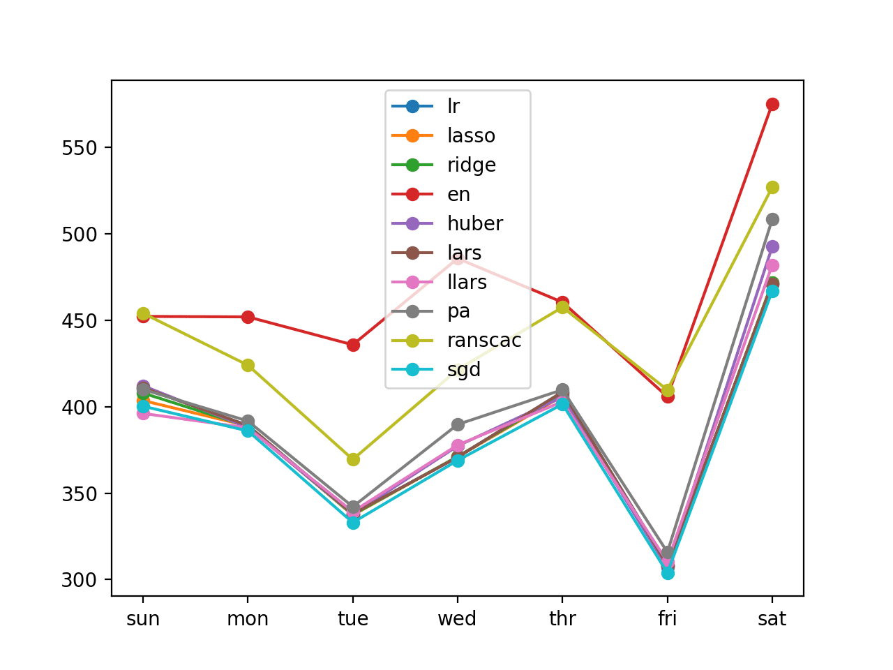
Line Plot of Recursive Multi-step Forecasts With Linear Algorithms
Better results may be achieved by tuning the hyperparameters of some of the better performing algorithms. Further, it may be interesting to update the example to test a suite of nonlinear and ensemble algorithms.
An interesting experiment may be to evaluate the performance of one or a few of the better performing algorithms with more or fewer prior days as input.
Direct Multi-Step Forecasting
An alternate to the recursive strategy for multi-step forecasting is to use a different model for each of the days to be forecasted.
This is called a direct multi-step forecasting strategy.
Because we are interested in forecasting seven days, this would require preparing seven different models, each specialized for forecasting a different day.
There are two approaches to training such a model:
- Predict Day. Models can be prepared to predict a specific day of the standard week, e.g. Monday.
- Predict Lead Time. Models can be prepared to predict a specific lead time, e.g. day 1.
Predicting a day will be more specific, but will mean that less of the training data can be used for each model. Predicting a lead time makes use of more of the training data, but requires the model to generalize across the different days of the week.
We will explore both approaches in this section.
Direct Day Approach
First, we must update the to_supervised() function to prepare the data, such as the prior week of observations, used as input and an observation from a specific day in the following week used as the output.
The updated to_supervised() function that implements this behavior is listed below. It takes an argument output_ix that defines the day [0,6] in the following week to use as the output.
# convert history into inputs and outputs
def to_supervised(history, output_ix):
	X, y = list(), list()
	# step over the entire history one time step at a time
	for i in range(len(history)-1):
		X.append(history[i][:,0])
		y.append(history[i + 1][output_ix,0])
	return array(X), array(y)
This function can be called seven times, once for each of the seven models required.
Next, we can update the sklearn_predict() function to create a new dataset and a new model for each day in the one-week forecast.
The body of the function is mostly unchanged, only it is used within a loop over each day in the output sequence, where the index of the day “i” is passed to the call to to_supervised() in order to prepare a specific dataset for training a model to predict that day.
The function no longer takes an n_input argument, as we have fixed the input to be the seven days of the prior week.
# fit a model and make a forecast
def sklearn_predict(model, history):
	yhat_sequence = list()
	# fit a model for each forecast day
	for i in range(7):
		# prepare data
		train_x, train_y = to_supervised(history, i)
		# make pipeline
		pipeline = make_pipeline(model)
		# fit the model
		pipeline.fit(train_x, train_y)
		# forecast
		x_input = array(train_x[-1, :]).reshape(1,7)
		yhat = pipeline.predict(x_input)[0]
		# store
		yhat_sequence.append(yhat)
	return yhat_sequence
The complete example is listed below.
# direct multi-step forecast by day
from math import sqrt
from numpy import split
from numpy import array
from pandas import read_csv
from sklearn.metrics import mean_squared_error
from matplotlib import pyplot
from sklearn.preprocessing import StandardScaler
from sklearn.preprocessing import MinMaxScaler
from sklearn.pipeline import Pipeline
from sklearn.linear_model import LinearRegression
from sklearn.linear_model import Lasso
from sklearn.linear_model import Ridge
from sklearn.linear_model import ElasticNet
from sklearn.linear_model import HuberRegressor
from sklearn.linear_model import Lars
from sklearn.linear_model import LassoLars
from sklearn.linear_model import PassiveAggressiveRegressor
from sklearn.linear_model import RANSACRegressor
from sklearn.linear_model import SGDRegressor

# split a univariate dataset into train/test sets
def split_dataset(data):
	# split into standard weeks
	train, test = data[1:-328], data[-328:-6]
	# restructure into windows of weekly data
	train = array(split(train, len(train)/7))
	test = array(split(test, len(test)/7))
	return train, test

# evaluate one or more weekly forecasts against expected values
def evaluate_forecasts(actual, predicted):
	scores = list()
	# calculate an RMSE score for each day
	for i in range(actual.shape[1]):
		# calculate mse
		mse = mean_squared_error(actual[:, i], predicted[:, i])
		# calculate rmse
		rmse = sqrt(mse)
		# store
		scores.append(rmse)
	# calculate overall RMSE
	s = 0
	for row in range(actual.shape[0]):
		for col in range(actual.shape[1]):
			s += (actual[row, col] - predicted[row, col])**2
	score = sqrt(s / (actual.shape[0] * actual.shape[1]))
	return score, scores

# summarize scores
def summarize_scores(name, score, scores):
	s_scores = ', '.join(['%.1f' % s for s in scores])
	print('%s: [%.3f] %s' % (name, score, s_scores))

# prepare a list of ml models
def get_models(models=dict()):
	# linear models
	models['lr'] = LinearRegression()
	models['lasso'] = Lasso()
	models['ridge'] = Ridge()
	models['en'] = ElasticNet()
	models['huber'] = HuberRegressor()
	models['lars'] = Lars()
	models['llars'] = LassoLars()
	models['pa'] = PassiveAggressiveRegressor(max_iter=1000, tol=1e-3)
	models['ranscac'] = RANSACRegressor()
	models['sgd'] = SGDRegressor(max_iter=1000, tol=1e-3)
	print('Defined %d models' % len(models))
	return models

# create a feature preparation pipeline for a model
def make_pipeline(model):
	steps = list()
	# standardization
	steps.append(('standardize', StandardScaler()))
	# normalization
	steps.append(('normalize', MinMaxScaler()))
	# the model
	steps.append(('model', model))
	# create pipeline
	pipeline = Pipeline(steps=steps)
	return pipeline

# convert history into inputs and outputs
def to_supervised(history, output_ix):
	X, y = list(), list()
	# step over the entire history one time step at a time
	for i in range(len(history)-1):
		X.append(history[i][:,0])
		y.append(history[i + 1][output_ix,0])
	return array(X), array(y)

# fit a model and make a forecast
def sklearn_predict(model, history):
	yhat_sequence = list()
	# fit a model for each forecast day
	for i in range(7):
		# prepare data
		train_x, train_y = to_supervised(history, i)
		# make pipeline
		pipeline = make_pipeline(model)
		# fit the model
		pipeline.fit(train_x, train_y)
		# forecast
		x_input = array(train_x[-1, :]).reshape(1,7)
		yhat = pipeline.predict(x_input)[0]
		# store
		yhat_sequence.append(yhat)
	return yhat_sequence

# evaluate a single model
def evaluate_model(model, train, test):
	# history is a list of weekly data
	history = [x for x in train]
	# walk-forward validation over each week
	predictions = list()
	for i in range(len(test)):
		# predict the week
		yhat_sequence = sklearn_predict(model, history)
		# store the predictions
		predictions.append(yhat_sequence)
		# get real observation and add to history for predicting the next week
		history.append(test[i, :])
	predictions = array(predictions)
	# evaluate predictions days for each week
	score, scores = evaluate_forecasts(test[:, :, 0], predictions)
	return score, scores

# load the new file
dataset = read_csv('household_power_consumption_days.csv', header=0, infer_datetime_format=True, parse_dates=['datetime'], index_col=['datetime'])
# split into train and test
train, test = split_dataset(dataset.values)
# prepare the models to evaluate
models = get_models()
# evaluate each model
days = ['sun', 'mon', 'tue', 'wed', 'thr', 'fri', 'sat']
for name, model in models.items():
	# evaluate and get scores
	score, scores = evaluate_model(model, train, test)
	# summarize scores
	summarize_scores(name, score, scores)
	# plot scores
	pyplot.plot(days, scores, marker='o', label=name)
# show plot
pyplot.legend()
pyplot.show()
Running the example first summarizes the performance of each model.
We can see that the performance is slightly worse than the recursive model on this problem.
Defined 10 models
lr: [410.927] 463.8, 381.4, 351.9, 430.7, 387.8, 350.4, 488.8
lasso: [408.440] 458.4, 378.5, 352.9, 429.5, 388.0, 348.0, 483.5
ridge: [403.875] 447.1, 377.9, 347.5, 427.4, 384.1, 343.4, 479.7
en: [454.263] 471.8, 433.8, 415.8, 477.4, 434.4, 373.8, 551.8
huber: [409.500] 466.8, 380.2, 359.8, 432.4, 387.0, 351.3, 470.9
lars: [410.927] 463.8, 381.4, 351.9, 430.7, 387.8, 350.4, 488.8
llars: [406.490] 453.0, 378.8, 357.3, 428.1, 388.0, 345.0, 476.9
pa: [402.476] 428.4, 380.9, 356.5, 426.7, 390.4, 348.6, 471.4
ranscac: [497.225] 456.1, 423.0, 445.9, 547.6, 521.9, 451.5, 607.2
sgd: [403.526] 441.4, 378.2, 354.5, 423.9, 382.4, 345.8, 480.3
A line plot of the per-day RMSE scores for each model is also created, showing a similar grouping of models as was seen with the recursive model.
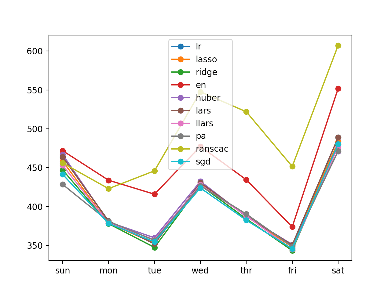
Line Plot of Direct Per-Day Multi-step Forecasts With Linear Algorithms
Direct Lead Time Approach
The direct lead time approach is the same, except that the to_supervised() makes use of more of the training dataset.
The function is the same as it was defined in the recursive model example, except it takes an additional output_ix argument to define the day in the following week to use as the output.
The updated to_supervised() function for the direct per-lead time strategy is listed below.
Unlike the per-day strategy, this version of the function does support variable sized inputs (not just seven days), allowing you to experiment if you like.
# convert history into inputs and outputs
def to_supervised(history, n_input, output_ix):
	# convert history to a univariate series
	data = to_series(history)
	X, y = list(), list()
	ix_start = 0
	# step over the entire history one time step at a time
	for i in range(len(data)):
		# define the end of the input sequence
		ix_end = ix_start + n_input
		ix_output = ix_end + output_ix
		# ensure we have enough data for this instance
		if ix_output < len(data):
			X.append(data[ix_start:ix_end])
			y.append(data[ix_output])
		# move along one time step
		ix_start += 1
	return array(X), array(y)
The complete example is listed below.
# direct multi-step forecast by lead time
from math import sqrt
from numpy import split
from numpy import array
from pandas import read_csv
from sklearn.metrics import mean_squared_error
from matplotlib import pyplot
from sklearn.preprocessing import StandardScaler
from sklearn.preprocessing import MinMaxScaler
from sklearn.pipeline import Pipeline
from sklearn.linear_model import LinearRegression
from sklearn.linear_model import Lasso
from sklearn.linear_model import Ridge
from sklearn.linear_model import ElasticNet
from sklearn.linear_model import HuberRegressor
from sklearn.linear_model import Lars
from sklearn.linear_model import LassoLars
from sklearn.linear_model import PassiveAggressiveRegressor
from sklearn.linear_model import RANSACRegressor
from sklearn.linear_model import SGDRegressor

# split a univariate dataset into train/test sets
def split_dataset(data):
	# split into standard weeks
	train, test = data[1:-328], data[-328:-6]
	# restructure into windows of weekly data
	train = array(split(train, len(train)/7))
	test = array(split(test, len(test)/7))
	return train, test

# evaluate one or more weekly forecasts against expected values
def evaluate_forecasts(actual, predicted):
	scores = list()
	# calculate an RMSE score for each day
	for i in range(actual.shape[1]):
		# calculate mse
		mse = mean_squared_error(actual[:, i], predicted[:, i])
		# calculate rmse
		rmse = sqrt(mse)
		# store
		scores.append(rmse)
	# calculate overall RMSE
	s = 0
	for row in range(actual.shape[0]):
		for col in range(actual.shape[1]):
			s += (actual[row, col] - predicted[row, col])**2
	score = sqrt(s / (actual.shape[0] * actual.shape[1]))
	return score, scores

# summarize scores
def summarize_scores(name, score, scores):
	s_scores = ', '.join(['%.1f' % s for s in scores])
	print('%s: [%.3f] %s' % (name, score, s_scores))

# prepare a list of ml models
def get_models(models=dict()):
	# linear models
	models['lr'] = LinearRegression()
	models['lasso'] = Lasso()
	models['ridge'] = Ridge()
	models['en'] = ElasticNet()
	models['huber'] = HuberRegressor()
	models['lars'] = Lars()
	models['llars'] = LassoLars()
	models['pa'] = PassiveAggressiveRegressor(max_iter=1000, tol=1e-3)
	models['ranscac'] = RANSACRegressor()
	models['sgd'] = SGDRegressor(max_iter=1000, tol=1e-3)
	print('Defined %d models' % len(models))
	return models

# create a feature preparation pipeline for a model
def make_pipeline(model):
	steps = list()
	# standardization
	steps.append(('standardize', StandardScaler()))
	# normalization
	steps.append(('normalize', MinMaxScaler()))
	# the model
	steps.append(('model', model))
	# create pipeline
	pipeline = Pipeline(steps=steps)
	return pipeline

# # convert windows of weekly multivariate data into a series of total power
def to_series(data):
	# extract just the total power from each week
	series = [week[:, 0] for week in data]
	# flatten into a single series
	series = array(series).flatten()
	return series

# convert history into inputs and outputs
def to_supervised(history, n_input, output_ix):
	# convert history to a univariate series
	data = to_series(history)
	X, y = list(), list()
	ix_start = 0
	# step over the entire history one time step at a time
	for i in range(len(data)):
		# define the end of the input sequence
		ix_end = ix_start + n_input
		ix_output = ix_end + output_ix
		# ensure we have enough data for this instance
		if ix_output < len(data):
			X.append(data[ix_start:ix_end])
			y.append(data[ix_output])
		# move along one time step
		ix_start += 1
	return array(X), array(y)

# fit a model and make a forecast
def sklearn_predict(model, history, n_input):
	yhat_sequence = list()
	# fit a model for each forecast day
	for i in range(7):
		# prepare data
		train_x, train_y = to_supervised(history, n_input, i)
		# make pipeline
		pipeline = make_pipeline(model)
		# fit the model
		pipeline.fit(train_x, train_y)
		# forecast
		x_input = array(train_x[-1, :]).reshape(1,n_input)
		yhat = pipeline.predict(x_input)[0]
		# store
		yhat_sequence.append(yhat)
	return yhat_sequence

# evaluate a single model
def evaluate_model(model, train, test, n_input):
	# history is a list of weekly data
	history = [x for x in train]
	# walk-forward validation over each week
	predictions = list()
	for i in range(len(test)):
		# predict the week
		yhat_sequence = sklearn_predict(model, history, n_input)
		# store the predictions
		predictions.append(yhat_sequence)
		# get real observation and add to history for predicting the next week
		history.append(test[i, :])
	predictions = array(predictions)
	# evaluate predictions days for each week
	score, scores = evaluate_forecasts(test[:, :, 0], predictions)
	return score, scores

# load the new file
dataset = read_csv('household_power_consumption_days.csv', header=0, infer_datetime_format=True, parse_dates=['datetime'], index_col=['datetime'])
# split into train and test
train, test = split_dataset(dataset.values)
# prepare the models to evaluate
models = get_models()
n_input = 7
# evaluate each model
days = ['sun', 'mon', 'tue', 'wed', 'thr', 'fri', 'sat']
for name, model in models.items():
	# evaluate and get scores
	score, scores = evaluate_model(model, train, test, n_input)
	# summarize scores
	summarize_scores(name, score, scores)
	# plot scores
	pyplot.plot(days, scores, marker='o', label=name)
# show plot
pyplot.legend()
pyplot.show()
Running the example summarizes the overall and per-day RMSE for each of the evaluated linear models.
We can see that generally the per-lead time approach resulted in better performance than the per-day version. This is likely because the approach made more of the training data available to the model.
Defined 10 models
lr: [394.983] 411.0, 400.7, 340.2, 382.9, 385.1, 362.8, 469.4
lasso: [391.767] 403.6, 394.4, 336.1, 382.7, 384.2, 360.4, 468.1
ridge: [393.444] 407.9, 397.8, 338.9, 383.2, 383.2, 360.4, 469.6
en: [461.986] 452.2, 448.3, 430.3, 480.4, 448.9, 396.0, 560.6
huber: [394.287] 412.1, 394.0, 333.4, 384.1, 383.1, 364.3, 474.4
lars: [394.983] 411.0, 400.7, 340.2, 382.9, 385.1, 362.8, 469.4
llars: [390.075] 396.1, 390.1, 334.3, 384.4, 385.2, 355.6, 470.9
pa: [389.340] 409.7, 380.6, 328.3, 388.6, 370.1, 351.8, 478.4
ranscac: [439.298] 387.2, 462.4, 394.4, 427.7, 412.9, 447.9, 526.8
sgd: [390.184] 396.7, 386.7, 337.6, 391.4, 374.0, 357.1, 473.5
A line plot of the per-day RMSE scores was again created.
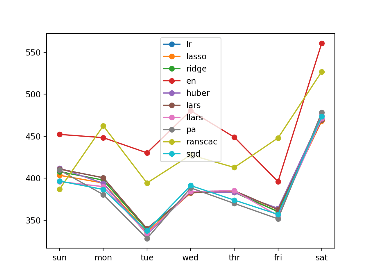
Line Plot of Direct Per-Lead Time Multi-step Forecasts With Linear Algorithms
It may be interesting to explore a blending of the per-day and per-time step approaches to modeling the problem.
It may also be interesting to see if increasing the number of prior days used as input for the per-lead time improves performance, e.g. using two weeks of data instead of one week.
Extensions
This section lists some ideas for extending the tutorial that you may wish to explore.
- Tune Models. Select one well-performing model and tune the model hyperparameters in order to further improve performance.
- Tune Data Preparation. All data was standardized and normalized prior to fitting each model; explore whether these methods are necessary and whether more or different combinations of data scaling methods can result in better performance.
- Explore Input Size. The input size was limited to seven days of prior observations; explore more and fewer days of observations as input and their impact on model performance.
- Nonlinear Algorithms. Explore a suite of nonlinear and ensemble machine learning algorithms to see if they can lift performance, such as SVM and Random Forest.
- Multivariate Direct Models. Develop direct models that make use of all input variables for the prior week, not just the total daily power consumed. This will require flattening the 2D arrays of seven days of eight variables into 1D vectors.
If you explore any of these extensions, I’d love to know.
Further Reading
This section provides more resources on the topic if you are looking to go deeper.
API
- pandas.read_csv API
- pandas.DataFrame.resample API
- Resample Offset Aliases
- sklearn.metrics.mean_squared_error API
- numpy.split API
Articles
- Individual household electric power consumption Data Set, UCI Machine Learning Repository.
- AC power, Wikipedia.
- 4 Strategies for Multi-Step Time Series Forecasting
Summary
In this tutorial, you discovered how to develop recursive and direct multi-step forecasting models with machine learning algorithms.
Specifically, you learned:
- How to develop a framework for evaluating linear, nonlinear, and ensemble machine learning algorithms for multi-step time series forecasting.
- How to evaluate machine learning algorithms using a recursive multi-step time series forecasting strategy.
- How to evaluate machine learning algorithms using a direct per-day and per-lead time multi-step time series forecasting strategy.
Do you have any questions?
Ask your questions in the comments below and I will do my best to answer.
The post Multi-step Time Series Forecasting with Machine Learning for Household Electricity Consumption appeared first on Machine Learning Mastery.