
Author: Jason Brownlee
Real-world time series forecasting is challenging for a whole host of reasons not limited to problem features such as having multiple input variables, the requirement to predict multiple time steps, and the need to perform the same type of prediction for multiple physical sites.
The EMC Data Science Global Hackathon dataset, or the ‘Air Quality Prediction’ dataset for short, describes weather conditions at multiple sites and requires a prediction of air quality measurements over the subsequent three days.
Machine learning algorithms can be applied to time series forecasting problems and offer benefits such as the ability to handle multiple input variables with noisy complex dependencies.
In this tutorial, you will discover how to develop machine learning models for multi-step time series forecasting of air pollution data.
After completing this tutorial, you will know:
- How to impute missing values and transform time series data so that it can be modeled by supervised learning algorithms.
- How to develop and evaluate a suite of linear algorithms for multi-step time series forecasting.
- How to develop and evaluate a suite of nonlinear algorithms for multi-step time series forecasting.
Let’s get started.

How to Develop Machine Learning Models for Multivariate Multi-Step Air Pollution Time Series Forecasting
Photo by Eric Schmuttenmaer, some rights reserved.
Tutorial Overview
This tutorial is divided into nine parts; they are:
- Problem Description
- Model Evaluation
- Machine Learning Modeling
- Machine Learning Data Preparation
- Model Evaluation Test Harness
- Evaluate Linear Algorithms
- Evaluate Nonlinear Algorithms
- Tune Lag Size
Problem Description
The Air Quality Prediction dataset describes weather conditions at multiple sites and requires a prediction of air quality measurements over the subsequent three days.
Specifically, weather observations such as temperature, pressure, wind speed, and wind direction are provided hourly for eight days for multiple sites. The objective is to predict air quality measurements for the next 3 days at multiple sites. The forecast lead times are not contiguous; instead, specific lead times must be forecast over the 72 hour forecast period. They are:
+1, +2, +3, +4, +5, +10, +17, +24, +48, +72
Further, the dataset is divided into disjoint but contiguous chunks of data, with eight days of data followed by three days that require a forecast.
Not all observations are available at all sites or chunks and not all output variables are available at all sites and chunks. There are large portions of missing data that must be addressed.
The dataset was used as the basis for a short duration machine learning competition (or hackathon) on the Kaggle website in 2012.
Submissions for the competition were evaluated against the true observations that were withheld from participants and scored using Mean Absolute Error (MAE). Submissions required the value of -1,000,000 to be specified in those cases where a forecast was not possible due to missing data. In fact, a template of where to insert missing values was provided and required to be adopted for all submissions (what a pain).
A winning entrant achieved a MAE of 0.21058 on the withheld test set (private leaderboard) using random forest on lagged observations. A writeup of this solution is available in the post:
- Chucking everything into a Random Forest: Ben Hamner on Winning The Air Quality Prediction Hackathon, 2012.
In this tutorial, we will explore how to develop naive forecasts for the problem that can be used as a baseline to determine whether a model has skill on the problem or not.
Need help with Deep Learning for Time Series?
Take my free 7-day email crash course now (with sample code).
Click to sign-up and also get a free PDF Ebook version of the course.
Model Evaluation
Before we can evaluate naive forecasting methods, we must develop a test harness.
This includes at least how the data will be prepared and how forecasts will be evaluated.
Load Dataset
The first step is to download the dataset and load it into memory.
The dataset can be downloaded for free from the Kaggle website. You may have to create an account and log in, in order to be able to download the dataset.
Download the entire dataset, e.g. “Download All” to your workstation and unzip the archive in your current working directory with the folder named ‘AirQualityPrediction‘.
Our focus will be the ‘TrainingData.csv‘ file that contains the training dataset, specifically data in chunks where each chunk is eight contiguous days of observations and target variables.
We can load the data file into memory using the Pandas read_csv() function and specify the header row on line 0.
# load dataset
dataset = read_csv('AirQualityPrediction/TrainingData.csv', header=0)
We can group data by the ‘chunkID’ variable (column index 1).
First, let’s get a list of the unique chunk identifiers.
chunk_ids = unique(values[:, 1])
We can then collect all rows for each chunk identifier and store them in a dictionary for easy access.
chunks = dict()
# sort rows by chunk id
for chunk_id in chunk_ids:
	selection = values[:, chunk_ix] == chunk_id
	chunks[chunk_id] = values[selection, :]
Below defines a function named to_chunks() that takes a NumPy array of the loaded data and returns a dictionary of chunk_id to rows for the chunk.
# split the dataset by 'chunkID', return a dict of id to rows
def to_chunks(values, chunk_ix=1):
	chunks = dict()
	# get the unique chunk ids
	chunk_ids = unique(values[:, chunk_ix])
	# group rows by chunk id
	for chunk_id in chunk_ids:
		selection = values[:, chunk_ix] == chunk_id
		chunks[chunk_id] = values[selection, :]
	return chunks
The complete example that loads the dataset and splits it into chunks is listed below.
# load data and split into chunks
from numpy import unique
from pandas import read_csv

# split the dataset by 'chunkID', return a dict of id to rows
def to_chunks(values, chunk_ix=1):
	chunks = dict()
	# get the unique chunk ids
	chunk_ids = unique(values[:, chunk_ix])
	# group rows by chunk id
	for chunk_id in chunk_ids:
		selection = values[:, chunk_ix] == chunk_id
		chunks[chunk_id] = values[selection, :]
	return chunks

# load dataset
dataset = read_csv('AirQualityPrediction/TrainingData.csv', header=0)
# group data by chunks
values = dataset.values
chunks = to_chunks(values)
print('Total Chunks: %d' % len(chunks))
Running the example prints the number of chunks in the dataset.
Total Chunks: 208
Data Preparation
Now that we know how to load the data and split it into chunks, we can separate into train and test datasets.
Each chunk covers an interval of eight days of hourly observations, although the number of actual observations within each chunk may vary widely.
We can split each chunk into the first five days of observations for training and the last three for test.
Each observation has a row called ‘position_within_chunk‘ that varies from 1 to 192 (8 days * 24 hours). We can therefore take all rows with a value in this column that is less than or equal to 120 (5 * 24) as training data and any values more than 120 as test data.
Further, any chunks that don’t have any observations in the train or test split can be dropped as not viable.
When working with the naive models, we are only interested in the target variables, and none of the input meteorological variables. Therefore, we can remove the input data and have the train and test data only comprised of the 39 target variables for each chunk, as well as the position within chunk and hour of observation.
The split_train_test() function below implements this behavior; given a dictionary of chunks, it will split each into a list of train and test chunk data.
# split each chunk into train/test sets
def split_train_test(chunks, row_in_chunk_ix=2):
	train, test = list(), list()
	# first 5 days of hourly observations for train
	cut_point = 5 * 24
	# enumerate chunks
	for k,rows in chunks.items():
		# split chunk rows by 'position_within_chunk'
		train_rows = rows[rows[:,row_in_chunk_ix] <= cut_point, :]
		test_rows = rows[rows[:,row_in_chunk_ix] > cut_point, :]
		if len(train_rows) == 0 or len(test_rows) == 0:
			print('>dropping chunk=%d: train=%s, test=%s' % (k, train_rows.shape, test_rows.shape))
			continue
		# store with chunk id, position in chunk, hour and all targets
		indices = [1,2,5] + [x for x in range(56,train_rows.shape[1])]
		train.append(train_rows[:, indices])
		test.append(test_rows[:, indices])
	return train, test
We do not require the entire test dataset; instead, we only require the observations at specific lead times over the three day period, specifically the lead times:
+1, +2, +3, +4, +5, +10, +17, +24, +48, +72
Where, each lead time is relative to the end of the training period.
First, we can put these lead times into a function for easy reference:
# return a list of relative forecast lead times
def get_lead_times():
	return [1, 2 ,3, 4, 5, 10, 17, 24, 48, 72]
Next, we can reduce the test dataset down to just the data at the preferred lead times.
We can do that by looking at the ‘position_within_chunk‘ column and using the lead time as an offset from the end of the training dataset, e.g. 120 + 1, 120 +2, etc.
If we find a matching row in the test set, it is saved, otherwise a row of NaN observations is generated.
The function to_forecasts() below implements this and returns a NumPy array with one row for each forecast lead time for each chunk.
# convert the rows in a test chunk to forecasts
def to_forecasts(test_chunks, row_in_chunk_ix=1):
	# get lead times
	lead_times = get_lead_times()
	# first 5 days of hourly observations for train
	cut_point = 5 * 24
	forecasts = list()
	# enumerate each chunk
	for rows in test_chunks:
		chunk_id = rows[0, 0]
		# enumerate each lead time
		for tau in lead_times:
			# determine the row in chunk we want for the lead time
			offset = cut_point + tau
			# retrieve data for the lead time using row number in chunk
			row_for_tau = rows[rows[:,row_in_chunk_ix]==offset, :]
			# check if we have data
			if len(row_for_tau) == 0:
				# create a mock row [chunk, position, hour] + [nan...]
				row = [chunk_id, offset, nan] + [nan for _ in range(39)]
				forecasts.append(row)
			else:
				# store the forecast row
				forecasts.append(row_for_tau[0])
	return array(forecasts)
We can tie all of this together and split the dataset into train and test sets and save the results to new files.
The complete code example is listed below.
# split data into train and test sets
from numpy import unique
from numpy import nan
from numpy import array
from numpy import savetxt
from pandas import read_csv

# split the dataset by 'chunkID', return a dict of id to rows
def to_chunks(values, chunk_ix=1):
	chunks = dict()
	# get the unique chunk ids
	chunk_ids = unique(values[:, chunk_ix])
	# group rows by chunk id
	for chunk_id in chunk_ids:
		selection = values[:, chunk_ix] == chunk_id
		chunks[chunk_id] = values[selection, :]
	return chunks

# split each chunk into train/test sets
def split_train_test(chunks, row_in_chunk_ix=2):
	train, test = list(), list()
	# first 5 days of hourly observations for train
	cut_point = 5 * 24
	# enumerate chunks
	for k,rows in chunks.items():
		# split chunk rows by 'position_within_chunk'
		train_rows = rows[rows[:,row_in_chunk_ix] <= cut_point, :]
		test_rows = rows[rows[:,row_in_chunk_ix] > cut_point, :]
		if len(train_rows) == 0 or len(test_rows) == 0:
			print('>dropping chunk=%d: train=%s, test=%s' % (k, train_rows.shape, test_rows.shape))
			continue
		# store with chunk id, position in chunk, hour and all targets
		indices = [1,2,5] + [x for x in range(56,train_rows.shape[1])]
		train.append(train_rows[:, indices])
		test.append(test_rows[:, indices])
	return train, test

# return a list of relative forecast lead times
def get_lead_times():
	return [1, 2 ,3, 4, 5, 10, 17, 24, 48, 72]

# convert the rows in a test chunk to forecasts
def to_forecasts(test_chunks, row_in_chunk_ix=1):
	# get lead times
	lead_times = get_lead_times()
	# first 5 days of hourly observations for train
	cut_point = 5 * 24
	forecasts = list()
	# enumerate each chunk
	for rows in test_chunks:
		chunk_id = rows[0, 0]
		# enumerate each lead time
		for tau in lead_times:
			# determine the row in chunk we want for the lead time
			offset = cut_point + tau
			# retrieve data for the lead time using row number in chunk
			row_for_tau = rows[rows[:,row_in_chunk_ix]==offset, :]
			# check if we have data
			if len(row_for_tau) == 0:
				# create a mock row [chunk, position, hour] + [nan...]
				row = [chunk_id, offset, nan] + [nan for _ in range(39)]
				forecasts.append(row)
			else:
				# store the forecast row
				forecasts.append(row_for_tau[0])
	return array(forecasts)

# load dataset
dataset = read_csv('AirQualityPrediction/TrainingData.csv', header=0)
# group data by chunks
values = dataset.values
chunks = to_chunks(values)
# split into train/test
train, test = split_train_test(chunks)
# flatten training chunks to rows
train_rows = array([row for rows in train for row in rows])
# print(train_rows.shape)
print('Train Rows: %s' % str(train_rows.shape))
# reduce train to forecast lead times only
test_rows = to_forecasts(test)
print('Test Rows: %s' % str(test_rows.shape))
# save datasets
savetxt('AirQualityPrediction/naive_train.csv', train_rows, delimiter=',')
savetxt('AirQualityPrediction/naive_test.csv', test_rows, delimiter=',')
Running the example first comments that chunk 69 is removed from the dataset for having insufficient data.
We can then see that we have 42 columns in each of the train and test sets, one for the chunk id, position within chunk, hour of day, and the 39 training variables.
We can also see the dramatically smaller version of the test dataset with rows only at the forecast lead times.
The new train and test datasets are saved in the ‘naive_train.csv‘ and ‘naive_test.csv‘ files respectively.
>dropping chunk=69: train=(0, 95), test=(28, 95)
Train Rows: (23514, 42)
Test Rows: (2070, 42)
Forecast Evaluation
Once forecasts have been made, they need to be evaluated.
It is helpful to have a simpler format when evaluating forecasts. For example, we will use the three-dimensional structure of [chunks][variables][time], where variable is the target variable number from 0 to 38 and time is the lead time index from 0 to 9.
Models are expected to make predictions in this format.
We can also restructure the test dataset to have this dataset for comparison. The prepare_test_forecasts() function below implements this.
# convert the test dataset in chunks to [chunk][variable][time] format
def prepare_test_forecasts(test_chunks):
	predictions = list()
	# enumerate chunks to forecast
	for rows in test_chunks:
		# enumerate targets for chunk
		chunk_predictions = list()
		for j in range(3, rows.shape[1]):
			yhat = rows[:, j]
			chunk_predictions.append(yhat)
		chunk_predictions = array(chunk_predictions)
		predictions.append(chunk_predictions)
	return array(predictions)
We will evaluate a model using the mean absolute error, or MAE. This is the metric that was used in the competition and is a sensible choice given the non-Gaussian distribution of the target variables.
If a lead time contains no data in the test set (e.g. NaN), then no error will be calculated for that forecast. If the lead time does have data in the test set but no data in the forecast, then the full magnitude of the observation will be taken as error. Finally, if the test set has an observation and a forecast was made, then the absolute difference will be recorded as the error.
The calculate_error() function implements these rules and returns the error for a given forecast.
# calculate the error between an actual and predicted value
def calculate_error(actual, predicted):
	# give the full actual value if predicted is nan
	if isnan(predicted):
		return abs(actual)
	# calculate abs difference
	return abs(actual - predicted)
Errors are summed across all chunks and all lead times, then averaged.
The overall MAE will be calculated, but we will also calculate a MAE for each forecast lead time. This can help with model selection generally as some models may perform differently at different lead times.
The evaluate_forecasts() function below implements this, calculating the MAE and per-lead time MAE for the provided predictions and expected values in [chunk][variable][time] format.
# evaluate a forecast in the format [chunk][variable][time]
def evaluate_forecasts(predictions, testset):
	lead_times = get_lead_times()
	total_mae, times_mae = 0.0, [0.0 for _ in range(len(lead_times))]
	total_c, times_c = 0, [0 for _ in range(len(lead_times))]
	# enumerate test chunks
	for i in range(len(test_chunks)):
		# convert to forecasts
		actual = testset[i]
		predicted = predictions[i]
		# enumerate target variables
		for j in range(predicted.shape[0]):
			# enumerate lead times
			for k in range(len(lead_times)):
				# skip if actual in nan
				if isnan(actual[j, k]):
					continue
				# calculate error
				error = calculate_error(actual[j, k], predicted[j, k])
				# update statistics
				total_mae += error
				times_mae[k] += error
				total_c += 1
				times_c[k] += 1
	# normalize summed absolute errors
	total_mae /= total_c
	times_mae = [times_mae[i]/times_c[i] for i in range(len(times_mae))]
	return total_mae, times_mae
Once we have the evaluation of a model, we can present it.
The summarize_error() function below first prints a one-line summary of a model’s performance then creates a plot of MAE per forecast lead time.
# summarize scores
def summarize_error(name, total_mae, times_mae):
	# print summary
	lead_times = get_lead_times()
	formatted = ['+%d %.3f' % (lead_times[i], times_mae[i]) for i in range(len(lead_times))]
	s_scores = ', '.join(formatted)
	print('%s: [%.3f MAE] %s' % (name, total_mae, s_scores))
	# plot summary
	pyplot.plot([str(x) for x in lead_times], times_mae, marker='.')
	pyplot.show()
We are now ready to start exploring the performance of naive forecasting methods.
Machine Learning Modeling
The problem can be modeled with machine learning.
Most machine learning models do not directly support the notion of observations over time. Instead, the lag observations must be treated as input features in order to make predictions.
This is a benefit of machine learning algorithms for time series forecasting. Specifically, that they are able to support large numbers of input features. These could be lag observations for one or multiple input time series.
Other general benefits of machine learning algorithms for time series forecasting over classical methods include:
- Ability to support noisy features and noise in the relationships between variables.
- Ability to handle irrelevant features.
- Ability to support complex relationships between variables.
A challenge with this dataset is the need to make multi-step forecasts. There are two main approaches that machine learning methods can be used to make multi-step forecasts; they are:
- Direct. A separate model is developed to forecast each forecast lead time.
- Recursive. A single model is developed to make one-step forecasts, and the model is used recursively where prior forecasts are used as input to forecast the subsequent lead time.
The recursive approach can make sense when forecasting a short contiguous block of lead times, whereas the direct approach may make more sense when forecasting discontiguous lead times. The direct approach may be more appropriate for the air pollution forecast problem given that we are interested in forecasting a mixture of 10 contiguous and discontiguous lead times over a three-day period.
The dataset has 39 target variables, and we develop one model per target variable, per forecast lead time. That means that we require (39 * 10) 390 machine learning models.
Key to the use of machine learning algorithms for time series forecasting is the choice of input data. We can think about three main sources of data that can be used as input and mapped to each forecast lead time for a target variable; they are:
- Univariate data, e.g. lag observations from the target variable that is being forecasted.
- Multivariate data, e.g. lag observations from other variables (weather and targets).
- Metadata, e.g. data about the date or time being forecast.
Data can be drawn from across all chunks, providing a rich dataset for learning a mapping from inputs to the target forecast lead time.
The 39 target variables are actually comprised of 12 variables across 14 sites.
Because of the way the data is provided, the default approach to modeling is to treat each variable-site as independent. It may be possible to collapse data by variable and use the same models for a variable across multiple sites.
Some variables have been purposely mislabeled (e.g different data used variables with the same identifier). Nevertheless, perhaps these mislabeled variables can be identified and excluded from multi-site models.
Machine Learning Data Preparation
Before we can explore machine learning models of this dataset, we must prepare the data in such a way that we can fit models.
This requires two data preparation steps:
- Handling missing data.
- Preparing input-output patterns.
For now, we will focus on the 39 target variables and ignore the meteorological and metadata.
Handle Missing Data
Chunks are comprised of five days or less of hourly observations for 39 target variables.
Many of the chunks do not have all five days of data, and none of the chunks have data for all 39 target variables.
In those cases where a chunk has no data for a target variable, a forecast is not required.
In those cases where a chunk does have some data for a target variable, but not all five days worth, there will be gaps in the series. These gaps may be a few hours to over a day of observations in length, sometimes even longer.
Three candidate strategies for dealing with these gaps are as follows:
- Ignore the gaps.
- Use data without gaps.
- Fill the gaps.
We could ignore the gaps. A problem with this would be that that data would not be contiguous when splitting data into inputs and outputs. When training a model, the inputs will not be consistent, but could mean the last n hours of data, or data spread across the last n days. This inconsistency will make learning a mapping from inputs to outputs very noisy and perhaps more difficult for the model than it needs to be.
We could use only the data without gaps. This is a good option. A risk is that we may not have much or enough data with which to fit a model.
Finally, we could fill the gaps. This is called data imputation and there are many strategies that could be used to fill the gaps. Three methods that may perform well include:
- Persisting the last observed value forward (linear).
- Use the median value for the hour of day within the chunk.
- Use the median value for the hour of day across chunks.
In this tutorial, we will use the latter approach and fill the gaps by using the median for the time of day across chunks. This method seems to result in more training samples and better model performance after a little testing.
For a given variable, there may be missing observations defined by missing rows. Specifically, each observation has a ‘position_within_chunk‘. We expect each chunk in the training dataset to have 120 observations, with ‘positions_within_chunk‘ from 1 to 120 inclusively.
Therefore, we can create an array of 120 NaN values for each variable, mark all observations in the chunk using the ‘positions_within_chunk‘ values, and anything left will be marked NaN. We can then plot each variable and look for gaps.
The variable_to_series() function below will take the rows for a chunk and a given column index for the target variable and will return a series of 120 time steps for the variable with all available data marked with the value from the chunk.
# layout a variable with breaks in the data for missing positions
def variable_to_series(chunk_train, col_ix, n_steps=5*24):
	# lay out whole series
	data = [nan for _ in range(n_steps)]
	# mark all available data
	for i in range(len(chunk_train)):
		# get position in chunk
		position = int(chunk_train[i, 1] - 1)
		# store data
		data[position] = chunk_train[i, col_ix]
	return data
We need to calculate a parallel series of the hour of day for each chunk that we can use for imputing hour specific data for each variable in the chunk.
Given a series of partially filled hours of day, the interpolate_hours() function below will fill in the missing hours of day. It does this by finding the first marked hour, then counting forward, filling in the hour of day, then performing the same operation backwards.
# interpolate series of hours (in place) in 24 hour time
def interpolate_hours(hours):
	# find the first hour
	ix = -1
	for i in range(len(hours)):
		if not isnan(hours[i]):
			ix = i
			break
	# fill-forward
	hour = hours[ix]
	for i in range(ix+1, len(hours)):
		# increment hour
		hour += 1
		# check for a fill
		if isnan(hours[i]):
			hours[i] = hour % 24
	# fill-backward
	hour = hours[ix]
	for i in range(ix-1, -1, -1):
		# decrement hour
		hour -= 1
		# check for a fill
		if isnan(hours[i]):
			hours[i] = hour % 24
We can call the same variable_to_series() function (above) to create the series of hours with missing values (column index 2), then call interpolate_hours() to fill in the gaps.
# prepare sequence of hours for the chunk
hours = variable_to_series(rows, 2)
# interpolate hours
interpolate_hours(hours)
We can then pass the hours to any impute function that may make use of it.
We can now try filling in missing values in a chunk with values within the same series with the same hour. Specifically, we will find all rows with the same hour on the series and calculate the median value.
The impute_missing() below takes all of the rows in a chunk, the prepared sequence of hours of the day for the chunk, and the series with missing values for a variable and the column index for a variable.
It first checks to see if the series is all missing data and returns immediately if this is the case as no impute can be performed. It then enumerates over the time steps of the series and when it detects a time step with no data, it collects all rows in the series with data for the same hour and calculates the median value.
# impute missing data
def impute_missing(train_chunks, rows, hours, series, col_ix):
	# impute missing using the median value for hour in all series
	imputed = list()
	for i in range(len(series)):
		if isnan(series[i]):
			# collect all rows across all chunks for the hour
			all_rows = list()
			for rows in train_chunks:
				[all_rows.append(row) for row in rows[rows[:,2]==hours[i]]]
			# calculate the central tendency for target
			all_rows = array(all_rows)
			# fill with median value
			value = nanmedian(all_rows[:, col_ix])
			if isnan(value):
				value = 0.0
			imputed.append(value)
		else:
			imputed.append(series[i])
	return imputed
Supervised Representation
We need to transform the series for each target variable into rows with inputs and outputs so that we can fit supervised machine learning algorithms.
Specifically, we have a series, like:
[1, 2, 3, 4, 5, 6, 7, 8, 9]
When forecasting the lead time of +1 using 2 lag variables, we would split the series into input (X) and output (y) patterns as follows:
X,			y
1, 2,		3
2, 3,		4
3, 4,		5
4, 5,		6
5, 6,		7
6, 7,		8
7, 8,		9
This first requires that we choose a number of lag observations to use as input. There is no right answer; instead, it is a good idea to test different numbers and see what works.
We then must perform the splitting of the series into the supervised learning format for each of the 10 forecast lead times. For example, forecasting +24 with 2 lag observations might look like:
X,			y
1, 2,		24
This process is then repeated for each of the 39 target variables.
The patterns prepared for each lead time for each target variable can then be aggregated across chunks to provide a training dataset for a model.
We must also prepare a test dataset. That is, input data (X) for each target variable for each chunk so that we can use it as input to forecast the lead times in the test dataset. If we chose a lag of 2, then the test dataset would be comprised of the last two observations for each target variable for each chunk. Pretty straightforward.
We can start off by defining a function that will create input-output patterns for a given complete (imputed) series.
The supervised_for_lead_time() function below will take a series, a number of lag observations to use as input, and a forecast lead time to predict, then will return a list of input/out rows drawn from the series.
# created input/output patterns from a sequence
def supervised_for_lead_time(series, n_lag, lead_time):
	samples = list()
	# enumerate observations and create input/output patterns
	for i in range(n_lag, len(series)):
		end_ix = i + (lead_time - 1)
		# check if can create a pattern
		if end_ix >= len(series):
			break
		# retrieve input and output
		start_ix = i - n_lag
		row = series[start_ix:i] + [series[end_ix]]
		samples.append(row)
	return samples
It is important to understand this piece.
We can test this function and explore different numbers of lag variables and forecast lead times on a small test dataset.
Below is a complete example that generates a series of 20 integers and creates a series with two input lags and forecasts the +6 lead time.
# test supervised to input/output patterns
from numpy import array

# created input/output patterns from a sequence
def supervised_for_lead_time(series, n_lag, lead_time):
	data = list()
	# enumerate observations and create input/output patterns
	for i in range(n_lag, len(series)):
		end_ix = i + (lead_time - 1)
		# check if can create a pattern
		if end_ix >= len(series):
			break
		# retrieve input and output
		start_ix = i - n_lag
		row = series[start_ix:i] + [series[end_ix]]
		data.append(row)
	return array(data)

# define test dataset
data = [x for x in range(20)]
# convert to supervised format
result = supervised_for_lead_time(data, 2, 6)
# display result
print(result)
Running the example prints the resulting patterns showing lag observations and their associated forecast lead time.
Experiment with this example to get comfortable with this data transform as it is key to modeling time series using machine learning algorithms.
[[ 0  1  7]
 [ 1  2  8]
 [ 2  3  9]
 [ 3  4 10]
 [ 4  5 11]
 [ 5  6 12]
 [ 6  7 13]
 [ 7  8 14]
 [ 8  9 15]
 [ 9 10 16]
 [10 11 17]
 [11 12 18]
 [12 13 19]]
We can now call supervised_for_lead_time() for each forecast lead time for a given target variable series.
The target_to_supervised() function below implements this. First the target variable is converted into a series and imputed using the functions developed in the previous section. Then training samples are created for each target lead time. A test sample for the target variable is also created.
Both the training data for each forecast lead time and the test input data are then returned for this target variable.
# create supervised learning data for each lead time for this target
def target_to_supervised(chunks, rows, hours, col_ix, n_lag):
	train_lead_times = list()
	# get series
	series = variable_to_series(rows, col_ix)
	if not has_data(series):
		return None, [nan for _ in range(n_lag)]
	# impute
	imputed = impute_missing(chunks, rows, hours, series, col_ix)
	# prepare test sample for chunk-variable
	test_sample = array(imputed[-n_lag:])
	# enumerate lead times
	lead_times = get_lead_times()
	for lead_time in lead_times:
		# make input/output data from series
		train_samples = supervised_for_lead_time(imputed, n_lag, lead_time)
		train_lead_times.append(train_samples)
	return train_lead_times, test_sample
We have the pieces; we now need to define the function to drive the data preparation process.
This function builds up the train and test datasets.
The approach is to enumerate each target variable and gather the training data for each lead time from across all of the chunks. At the same time, we collect the samples required as input when making a prediction for the test dataset.
The result is a training dataset that has the dimensions [var][lead time][sample] where the final dimension are the rows of training samples for a forecast lead time for a target variable. The function also returns the test dataset with the dimensions [chunk][var][sample] where the final dimension is the input data for making a prediction for a target variable for a chunk.
The data_prep() function below implements this behavior and takes the data in chunk format and a specified number of lag observations to use as input.
# prepare training [var][lead time][sample] and test [chunk][var][sample]
def data_prep(chunks, n_lag, n_vars=39):
	lead_times = get_lead_times()
	train_data = [[list() for _ in range(len(lead_times))] for _ in range(n_vars)]
	test_data = [[list() for _ in range(n_vars)] for _ in range(len(chunks))]
	# enumerate targets for chunk
	for var in range(n_vars):
		# convert target number into column number
		col_ix = 3 + var
		# enumerate chunks to forecast
		for c_id in range(len(chunks)):
			rows = chunks[c_id]
			# prepare sequence of hours for the chunk
			hours = variable_to_series(rows, 2)
			# interpolate hours
			interpolate_hours(hours)
			# check for no data
			if not has_data(rows[:, col_ix]):
				continue
			# convert series into training data for each lead time
			train, test_sample = target_to_supervised(chunks, rows, hours, col_ix, n_lag)
			# store test sample for this var-chunk
			test_data[c_id][var] = test_sample
			if train is not None:
				# store samples per lead time
				for lead_time in range(len(lead_times)):
					# add all rows to the existing list of rows
					train_data[var][lead_time].extend(train[lead_time])
		# convert all rows for each var-lead time to a numpy array
		for lead_time in range(len(lead_times)):
			train_data[var][lead_time] = array(train_data[var][lead_time])
	return array(train_data), array(test_data)
Complete Example
We can tie everything together and prepare a train and test dataset with a supervised learning format for machine learning algorithms.
We will use the prior 12 hours of lag observations as input when predicting each forecast lead time.
The resulting train and test datasets are then saved as binary NumPy arrays.
The complete example is listed below.
# prepare data
from numpy import loadtxt
from numpy import nan
from numpy import isnan
from numpy import count_nonzero
from numpy import unique
from numpy import array
from numpy import nanmedian
from numpy import save

# split the dataset by 'chunkID', return a list of chunks
def to_chunks(values, chunk_ix=0):
	chunks = list()
	# get the unique chunk ids
	chunk_ids = unique(values[:, chunk_ix])
	# group rows by chunk id
	for chunk_id in chunk_ids:
		selection = values[:, chunk_ix] == chunk_id
		chunks.append(values[selection, :])
	return chunks

# return a list of relative forecast lead times
def get_lead_times():
	return [1, 2, 3, 4, 5, 10, 17, 24, 48, 72]

# interpolate series of hours (in place) in 24 hour time
def interpolate_hours(hours):
	# find the first hour
	ix = -1
	for i in range(len(hours)):
		if not isnan(hours[i]):
			ix = i
			break
	# fill-forward
	hour = hours[ix]
	for i in range(ix+1, len(hours)):
		# increment hour
		hour += 1
		# check for a fill
		if isnan(hours[i]):
			hours[i] = hour % 24
	# fill-backward
	hour = hours[ix]
	for i in range(ix-1, -1, -1):
		# decrement hour
		hour -= 1
		# check for a fill
		if isnan(hours[i]):
			hours[i] = hour % 24

# return true if the array has any non-nan values
def has_data(data):
	return count_nonzero(isnan(data)) < len(data)

# impute missing data
def impute_missing(train_chunks, rows, hours, series, col_ix):
	# impute missing using the median value for hour in all series
	imputed = list()
	for i in range(len(series)):
		if isnan(series[i]):
			# collect all rows across all chunks for the hour
			all_rows = list()
			for rows in train_chunks:
				[all_rows.append(row) for row in rows[rows[:,2]==hours[i]]]
			# calculate the central tendency for target
			all_rows = array(all_rows)
			# fill with median value
			value = nanmedian(all_rows[:, col_ix])
			if isnan(value):
				value = 0.0
			imputed.append(value)
		else:
			imputed.append(series[i])
	return imputed

# layout a variable with breaks in the data for missing positions
def variable_to_series(chunk_train, col_ix, n_steps=5*24):
	# lay out whole series
	data = [nan for _ in range(n_steps)]
	# mark all available data
	for i in range(len(chunk_train)):
		# get position in chunk
		position = int(chunk_train[i, 1] - 1)
		# store data
		data[position] = chunk_train[i, col_ix]
	return data

# created input/output patterns from a sequence
def supervised_for_lead_time(series, n_lag, lead_time):
	samples = list()
	# enumerate observations and create input/output patterns
	for i in range(n_lag, len(series)):
		end_ix = i + (lead_time - 1)
		# check if can create a pattern
		if end_ix >= len(series):
			break
		# retrieve input and output
		start_ix = i - n_lag
		row = series[start_ix:i] + [series[end_ix]]
		samples.append(row)
	return samples

# create supervised learning data for each lead time for this target
def target_to_supervised(chunks, rows, hours, col_ix, n_lag):
	train_lead_times = list()
	# get series
	series = variable_to_series(rows, col_ix)
	if not has_data(series):
		return None, [nan for _ in range(n_lag)]
	# impute
	imputed = impute_missing(chunks, rows, hours, series, col_ix)
	# prepare test sample for chunk-variable
	test_sample = array(imputed[-n_lag:])
	# enumerate lead times
	lead_times = get_lead_times()
	for lead_time in lead_times:
		# make input/output data from series
		train_samples = supervised_for_lead_time(imputed, n_lag, lead_time)
		train_lead_times.append(train_samples)
	return train_lead_times, test_sample

# prepare training [var][lead time][sample] and test [chunk][var][sample]
def data_prep(chunks, n_lag, n_vars=39):
	lead_times = get_lead_times()
	train_data = [[list() for _ in range(len(lead_times))] for _ in range(n_vars)]
	test_data = [[list() for _ in range(n_vars)] for _ in range(len(chunks))]
	# enumerate targets for chunk
	for var in range(n_vars):
		# convert target number into column number
		col_ix = 3 + var
		# enumerate chunks to forecast
		for c_id in range(len(chunks)):
			rows = chunks[c_id]
			# prepare sequence of hours for the chunk
			hours = variable_to_series(rows, 2)
			# interpolate hours
			interpolate_hours(hours)
			# check for no data
			if not has_data(rows[:, col_ix]):
				continue
			# convert series into training data for each lead time
			train, test_sample = target_to_supervised(chunks, rows, hours, col_ix, n_lag)
			# store test sample for this var-chunk
			test_data[c_id][var] = test_sample
			if train is not None:
				# store samples per lead time
				for lead_time in range(len(lead_times)):
					# add all rows to the existing list of rows
					train_data[var][lead_time].extend(train[lead_time])
		# convert all rows for each var-lead time to a numpy array
		for lead_time in range(len(lead_times)):
			train_data[var][lead_time] = array(train_data[var][lead_time])
	return array(train_data), array(test_data)

# load dataset
train = loadtxt('AirQualityPrediction/naive_train.csv', delimiter=',')
test = loadtxt('AirQualityPrediction/naive_test.csv', delimiter=',')
# group data by chunks
train_chunks = to_chunks(train)
test_chunks = to_chunks(test)
# convert training data into supervised learning data
n_lag = 12
train_data, test_data = data_prep(train_chunks, n_lag)
print(train_data.shape, test_data.shape)
# save train and test sets to file
save('AirQualityPrediction/supervised_train.npy', train_data)
save('AirQualityPrediction/supervised_test.npy', test_data)
Running the example may take a minute.
The result are two binary files containing the train and test datasets that we can load in the following sections for training and evaluating machine learning algorithms on the problem.
Model Evaluation Test Harness
Before we can start evaluating algorithms, we need some more elements of the test harness.
First, we need to be able to fit a scikit-learn model on training data. The fit_model() function below will make a clone of the model configuration and fit it on the provided training data. We will need to fit many (360) versions of each configured model, so this function will be called a lot.
# fit a single model
def fit_model(model, X, y):
	# clone the model configuration
	local_model = clone(model)
	# fit the model
	local_model.fit(X, y)
	return local_model
Next, we need to fit a model for each variable and forecast lead time combination.
We can do this by enumerating the training dataset first by the variables and then by the lead times. We can then fit a model and store it in a list of lists with the same structure, specifically: [var][time][model].
The fit_models() function below implements this.
# fit one model for each variable and each forecast lead time [var][time][model]
def fit_models(model, train):
	# prepare structure for saving models
	models = [[list() for _ in range(train.shape[1])] for _ in range(train.shape[0])]
	# enumerate vars
	for i in range(train.shape[0]):
		# enumerate lead times
		for j in range(train.shape[1]):
			# get data
			data = train[i, j]
			X, y = data[:, :-1], data[:, -1]
			# fit model
			local_model = fit_model(model, X, y)
			models[i][j].append(local_model)
	return models
Fitting models is the slow part and could benefit from being parallelized, such as with the Joblib library. This is left as an extension.
Once the models are fit, they can be used to make predictions for the test dataset.
The prepared test dataset is organized first by chunk, and then by target variable. Making predictions is fast and involves first checking that a prediction can be made (we have input data) and if so, using the appropriate models for the target variable. Each of the 10 forecast lead times for the variable will then be predicted with each of the direct models for those lead times.
The make_predictions() function below implements this, taking the list of lists of models and the loaded test dataset as arguments and returning an array of forecasts with the structure [chunks][var][time].
# return forecasts as [chunks][var][time]
def make_predictions(models, test):
	lead_times = get_lead_times()
	predictions = list()
	# enumerate chunks
	for i in range(test.shape[0]):
		# enumerate variables
		chunk_predictions = list()
		for j in range(test.shape[1]):
			# get the input pattern for this chunk and target
			pattern = test[i,j]
			# assume a nan forecast
			forecasts = array([nan for _ in range(len(lead_times))])
			# check we can make a forecast
			if has_data(pattern):
				pattern = pattern.reshape((1, len(pattern)))
				# forecast each lead time
				forecasts = list()
				for k in range(len(lead_times)):
					yhat = models[j][k][0].predict(pattern)
					forecasts.append(yhat[0])
				forecasts = array(forecasts)
			# save forecasts fore each lead time for this variable
			chunk_predictions.append(forecasts)
		# save forecasts for this chunk
		chunk_predictions = array(chunk_predictions)
		predictions.append(chunk_predictions)
	return array(predictions)
We need a list of models to evaluate.
We can define a generic get_models() function that is responsible for defining a dictionary of model-names mapped to configured scikit-learn model objects.
# prepare a list of ml models
def get_models(models=dict()):
	# ...
	return models
Finally, we need a function to drive the model evaluation process.
Given the dictionary of models, enumerate the models, first fitting the matrix of models on the training data, making predictions of the test dataset, evaluating the predictions, and summarizing the results.
The evaluate_models() function below implements this.
# evaluate a suite of models
def evaluate_models(models, train, test, actual):
	for name, model in models.items():
		# fit models
		fits = fit_models(model, train)
		# make predictions
		predictions = make_predictions(fits, test)
		# evaluate forecast
		total_mae, _ = evaluate_forecasts(predictions, actual)
		# summarize forecast
		summarize_error(name, total_mae)
We now have everything we need to evaluate machine learning models.
Evaluate Linear Algorithms
In this section, we will spot check a suite of linear machine learning algorithms.
Linear algorithms are those that assume that the output is a linear function of the input variables. This is much like the assumptions of classical time series forecasting models like ARIMA.
Spot checking means evaluating a suite of models in order to get a rough idea of what works. We are interested in any models that outperform a simple autoregression model AR(2) that achieves a MAE error of about 0.487.
We will test eight linear machine learning algorithms with their default configuration; specifically:
- Linear Regression
- Lasso Linear Regression
- Ridge Regression
- Elastic Net Regression
- Huber Regression
- Lasso Lars Linear Regression
- Passive Aggressive Regression
- Stochastic Gradient Descent Regression
We can define these models in the get_models() function.
# prepare a list of ml models
def get_models(models=dict()):
	# linear models
	models['lr'] = LinearRegression()
	models['lasso'] = Lasso()
	models['ridge'] = Ridge()
	models['en'] = ElasticNet()
	models['huber'] = HuberRegressor()
	models['llars'] = LassoLars()
	models['pa'] = PassiveAggressiveRegressor(max_iter=1000, tol=1e-3)
	models['sgd'] = SGDRegressor(max_iter=1000, tol=1e-3)
	print('Defined %d models' % len(models))
	return models
The complete code example is listed below.
# evaluate linear algorithms
from numpy import load
from numpy import loadtxt
from numpy import nan
from numpy import isnan
from numpy import count_nonzero
from numpy import unique
from numpy import array
from sklearn.base import clone
from sklearn.linear_model import LinearRegression
from sklearn.linear_model import Lasso
from sklearn.linear_model import Ridge
from sklearn.linear_model import ElasticNet
from sklearn.linear_model import HuberRegressor
from sklearn.linear_model import LassoLars
from sklearn.linear_model import PassiveAggressiveRegressor
from sklearn.linear_model import SGDRegressor

# split the dataset by 'chunkID', return a list of chunks
def to_chunks(values, chunk_ix=0):
	chunks = list()
	# get the unique chunk ids
	chunk_ids = unique(values[:, chunk_ix])
	# group rows by chunk id
	for chunk_id in chunk_ids:
		selection = values[:, chunk_ix] == chunk_id
		chunks.append(values[selection, :])
	return chunks

# return true if the array has any non-nan values
def has_data(data):
	return count_nonzero(isnan(data)) < len(data)

# return a list of relative forecast lead times
def get_lead_times():
	return [1, 2, 3, 4, 5, 10, 17, 24, 48, 72]

# fit a single model
def fit_model(model, X, y):
	# clone the model configuration
	local_model = clone(model)
	# fit the model
	local_model.fit(X, y)
	return local_model

# fit one model for each variable and each forecast lead time [var][time][model]
def fit_models(model, train):
	# prepare structure for saving models
	models = [[list() for _ in range(train.shape[1])] for _ in range(train.shape[0])]
	# enumerate vars
	for i in range(train.shape[0]):
		# enumerate lead times
		for j in range(train.shape[1]):
			# get data
			data = train[i, j]
			X, y = data[:, :-1], data[:, -1]
			# fit model
			local_model = fit_model(model, X, y)
			models[i][j].append(local_model)
	return models

# return forecasts as [chunks][var][time]
def make_predictions(models, test):
	lead_times = get_lead_times()
	predictions = list()
	# enumerate chunks
	for i in range(test.shape[0]):
		# enumerate variables
		chunk_predictions = list()
		for j in range(test.shape[1]):
			# get the input pattern for this chunk and target
			pattern = test[i,j]
			# assume a nan forecast
			forecasts = array([nan for _ in range(len(lead_times))])
			# check we can make a forecast
			if has_data(pattern):
				pattern = pattern.reshape((1, len(pattern)))
				# forecast each lead time
				forecasts = list()
				for k in range(len(lead_times)):
					yhat = models[j][k][0].predict(pattern)
					forecasts.append(yhat[0])
				forecasts = array(forecasts)
			# save forecasts for each lead time for this variable
			chunk_predictions.append(forecasts)
		# save forecasts for this chunk
		chunk_predictions = array(chunk_predictions)
		predictions.append(chunk_predictions)
	return array(predictions)

# convert the test dataset in chunks to [chunk][variable][time] format
def prepare_test_forecasts(test_chunks):
	predictions = list()
	# enumerate chunks to forecast
	for rows in test_chunks:
		# enumerate targets for chunk
		chunk_predictions = list()
		for j in range(3, rows.shape[1]):
			yhat = rows[:, j]
			chunk_predictions.append(yhat)
		chunk_predictions = array(chunk_predictions)
		predictions.append(chunk_predictions)
	return array(predictions)

# calculate the error between an actual and predicted value
def calculate_error(actual, predicted):
	# give the full actual value if predicted is nan
	if isnan(predicted):
		return abs(actual)
	# calculate abs difference
	return abs(actual - predicted)

# evaluate a forecast in the format [chunk][variable][time]
def evaluate_forecasts(predictions, testset):
	lead_times = get_lead_times()
	total_mae, times_mae = 0.0, [0.0 for _ in range(len(lead_times))]
	total_c, times_c = 0, [0 for _ in range(len(lead_times))]
	# enumerate test chunks
	for i in range(len(test_chunks)):
		# convert to forecasts
		actual = testset[i]
		predicted = predictions[i]
		# enumerate target variables
		for j in range(predicted.shape[0]):
			# enumerate lead times
			for k in range(len(lead_times)):
				# skip if actual in nan
				if isnan(actual[j, k]):
					continue
				# calculate error
				error = calculate_error(actual[j, k], predicted[j, k])
				# update statistics
				total_mae += error
				times_mae[k] += error
				total_c += 1
				times_c[k] += 1
	# normalize summed absolute errors
	total_mae /= total_c
	times_mae = [times_mae[i]/times_c[i] for i in range(len(times_mae))]
	return total_mae, times_mae

# summarize scores
def summarize_error(name, total_mae):
	print('%s: %.3f MAE' % (name, total_mae))

# prepare a list of ml models
def get_models(models=dict()):
	# linear models
	models['lr'] = LinearRegression()
	models['lasso'] = Lasso()
	models['ridge'] = Ridge()
	models['en'] = ElasticNet()
	models['huber'] = HuberRegressor()
	models['llars'] = LassoLars()
	models['pa'] = PassiveAggressiveRegressor(max_iter=1000, tol=1e-3)
	models['sgd'] = SGDRegressor(max_iter=1000, tol=1e-3)
	print('Defined %d models' % len(models))
	return models

# evaluate a suite of models
def evaluate_models(models, train, test, actual):
	for name, model in models.items():
		# fit models
		fits = fit_models(model, train)
		# make predictions
		predictions = make_predictions(fits, test)
		# evaluate forecast
		total_mae, _ = evaluate_forecasts(predictions, actual)
		# summarize forecast
		summarize_error(name, total_mae)

# load supervised datasets
train = load('AirQualityPrediction/supervised_train.npy')
test = load('AirQualityPrediction/supervised_test.npy')
print(train.shape, test.shape)
# load test chunks for validation
testset = loadtxt('AirQualityPrediction/naive_test.csv', delimiter=',')
test_chunks = to_chunks(testset)
actual = prepare_test_forecasts(test_chunks)
# prepare list of models
models = get_models()
# evaluate models
evaluate_models(models, train, test, actual)
Running the example prints the MAE for each of the evaluated algorithms.
We can see that many of the algorithms show skill compared to a simple AR model, achieving a MAE below 0.487.
Huber regression seems to perform the best (with default configuration), achieving a MAE of 0.434.
This is interesting as Huber regression, or robust regression with Huber loss, is a method that is designed to be robust to outliers in the training dataset. It may suggest that the other methods may perform better with a little more data preparation, such as standardization and/or outlier removal.
lr: 0.454 MAE
lasso: 0.624 MAE
ridge: 0.454 MAE
en: 0.595 MAE
huber: 0.434 MAE
llars: 0.631 MAE
pa: 0.833 MAE
sgd: 0.457 MAE
Nonlinear Algorithms
We can use the same framework to evaluate the performance of a suite of nonlinear and ensemble machine learning algorithms.
Specifically:
Nonlinear Algorithms
- k-Nearest Neighbors
- Classification and Regression Trees
- Extra Tree
- Support Vector Regression
Ensemble Algorithms
- Adaboost
- Bagged Decision Trees
- Random Forest
- Extra Trees
- Gradient Boosting Machines
The get_models() function below defines these nine models.
# prepare a list of ml models
def get_models(models=dict()):
	# non-linear models
	models['knn'] = KNeighborsRegressor(n_neighbors=7)
	models['cart'] = DecisionTreeRegressor()
	models['extra'] = ExtraTreeRegressor()
	models['svmr'] = SVR()
	# # ensemble models
	n_trees = 100
	models['ada'] = AdaBoostRegressor(n_estimators=n_trees)
	models['bag'] = BaggingRegressor(n_estimators=n_trees)
	models['rf'] = RandomForestRegressor(n_estimators=n_trees)
	models['et'] = ExtraTreesRegressor(n_estimators=n_trees)
	models['gbm'] = GradientBoostingRegressor(n_estimators=n_trees)
	print('Defined %d models' % len(models))
	return models
The complete code listing is provided below.
# spot check nonlinear algorithms
from numpy import load
from numpy import loadtxt
from numpy import nan
from numpy import isnan
from numpy import count_nonzero
from numpy import unique
from numpy import array
from sklearn.base import clone
from sklearn.neighbors import KNeighborsRegressor
from sklearn.tree import DecisionTreeRegressor
from sklearn.tree import ExtraTreeRegressor
from sklearn.svm import SVR
from sklearn.ensemble import AdaBoostRegressor
from sklearn.ensemble import BaggingRegressor
from sklearn.ensemble import RandomForestRegressor
from sklearn.ensemble import ExtraTreesRegressor
from sklearn.ensemble import GradientBoostingRegressor

# split the dataset by 'chunkID', return a list of chunks
def to_chunks(values, chunk_ix=0):
	chunks = list()
	# get the unique chunk ids
	chunk_ids = unique(values[:, chunk_ix])
	# group rows by chunk id
	for chunk_id in chunk_ids:
		selection = values[:, chunk_ix] == chunk_id
		chunks.append(values[selection, :])
	return chunks

# return true if the array has any non-nan values
def has_data(data):
	return count_nonzero(isnan(data)) < len(data)

# return a list of relative forecast lead times
def get_lead_times():
	return [1, 2, 3, 4, 5, 10, 17, 24, 48, 72]

# fit a single model
def fit_model(model, X, y):
	# clone the model configuration
	local_model = clone(model)
	# fit the model
	local_model.fit(X, y)
	return local_model

# fit one model for each variable and each forecast lead time [var][time][model]
def fit_models(model, train):
	# prepare structure for saving models
	models = [[list() for _ in range(train.shape[1])] for _ in range(train.shape[0])]
	# enumerate vars
	for i in range(train.shape[0]):
		# enumerate lead times
		for j in range(train.shape[1]):
			# get data
			data = train[i, j]
			X, y = data[:, :-1], data[:, -1]
			# fit model
			local_model = fit_model(model, X, y)
			models[i][j].append(local_model)
	return models

# return forecasts as [chunks][var][time]
def make_predictions(models, test):
	lead_times = get_lead_times()
	predictions = list()
	# enumerate chunks
	for i in range(test.shape[0]):
		# enumerate variables
		chunk_predictions = list()
		for j in range(test.shape[1]):
			# get the input pattern for this chunk and target
			pattern = test[i,j]
			# assume a nan forecast
			forecasts = array([nan for _ in range(len(lead_times))])
			# check we can make a forecast
			if has_data(pattern):
				pattern = pattern.reshape((1, len(pattern)))
				# forecast each lead time
				forecasts = list()
				for k in range(len(lead_times)):
					yhat = models[j][k][0].predict(pattern)
					forecasts.append(yhat[0])
				forecasts = array(forecasts)
			# save forecasts for each lead time for this variable
			chunk_predictions.append(forecasts)
		# save forecasts for this chunk
		chunk_predictions = array(chunk_predictions)
		predictions.append(chunk_predictions)
	return array(predictions)

# convert the test dataset in chunks to [chunk][variable][time] format
def prepare_test_forecasts(test_chunks):
	predictions = list()
	# enumerate chunks to forecast
	for rows in test_chunks:
		# enumerate targets for chunk
		chunk_predictions = list()
		for j in range(3, rows.shape[1]):
			yhat = rows[:, j]
			chunk_predictions.append(yhat)
		chunk_predictions = array(chunk_predictions)
		predictions.append(chunk_predictions)
	return array(predictions)

# calculate the error between an actual and predicted value
def calculate_error(actual, predicted):
	# give the full actual value if predicted is nan
	if isnan(predicted):
		return abs(actual)
	# calculate abs difference
	return abs(actual - predicted)

# evaluate a forecast in the format [chunk][variable][time]
def evaluate_forecasts(predictions, testset):
	lead_times = get_lead_times()
	total_mae, times_mae = 0.0, [0.0 for _ in range(len(lead_times))]
	total_c, times_c = 0, [0 for _ in range(len(lead_times))]
	# enumerate test chunks
	for i in range(len(test_chunks)):
		# convert to forecasts
		actual = testset[i]
		predicted = predictions[i]
		# enumerate target variables
		for j in range(predicted.shape[0]):
			# enumerate lead times
			for k in range(len(lead_times)):
				# skip if actual in nan
				if isnan(actual[j, k]):
					continue
				# calculate error
				error = calculate_error(actual[j, k], predicted[j, k])
				# update statistics
				total_mae += error
				times_mae[k] += error
				total_c += 1
				times_c[k] += 1
	# normalize summed absolute errors
	total_mae /= total_c
	times_mae = [times_mae[i]/times_c[i] for i in range(len(times_mae))]
	return total_mae, times_mae

# summarize scores
def summarize_error(name, total_mae):
	print('%s: %.3f MAE' % (name, total_mae))

# prepare a list of ml models
def get_models(models=dict()):
	# non-linear models
	models['knn'] = KNeighborsRegressor(n_neighbors=7)
	models['cart'] = DecisionTreeRegressor()
	models['extra'] = ExtraTreeRegressor()
	models['svmr'] = SVR()
	# # ensemble models
	n_trees = 100
	models['ada'] = AdaBoostRegressor(n_estimators=n_trees)
	models['bag'] = BaggingRegressor(n_estimators=n_trees)
	models['rf'] = RandomForestRegressor(n_estimators=n_trees)
	models['et'] = ExtraTreesRegressor(n_estimators=n_trees)
	models['gbm'] = GradientBoostingRegressor(n_estimators=n_trees)
	print('Defined %d models' % len(models))
	return models

# evaluate a suite of models
def evaluate_models(models, train, test, actual):
	for name, model in models.items():
		# fit models
		fits = fit_models(model, train)
		# make predictions
		predictions = make_predictions(fits, test)
		# evaluate forecast
		total_mae, _ = evaluate_forecasts(predictions, actual)
		# summarize forecast
		summarize_error(name, total_mae)

# load supervised datasets
train = load('AirQualityPrediction/supervised_train.npy')
test = load('AirQualityPrediction/supervised_test.npy')
print(train.shape, test.shape)
# load test chunks for validation
testset = loadtxt('AirQualityPrediction/naive_test.csv', delimiter=',')
test_chunks = to_chunks(testset)
actual = prepare_test_forecasts(test_chunks)
# prepare list of models
models = get_models()
# evaluate models
evaluate_models(models, train, test, actual)
Running the example, we can see that many algorithms performed well compared to the baseline of an autoregression algorithm, although none performed as well as Huber regression in the previous section.
Both support vector regression and perhaps gradient boosting machines may be worth further investigation of achieving MAEs of 0.437 and 0.450 respectively.
knn: 0.484 MAE
cart: 0.631 MAE
extra: 0.630 MAE
svmr: 0.437 MAE
ada: 0.717 MAE
bag: 0.471 MAE
rf: 0.470 MAE
et: 0.469 MAE
gbm: 0.450 MAE
Tune Lag Size
In the previous spot check experiments, the number of lag observations was arbitrarily fixed at 12.
We can vary the number of lag observations and evaluate the effect on MAE. Some algorithms may require more or fewer prior observations, but general trends may hold across algorithms.
Prepare the supervised learning dataset with a range of different numbers of lag observations and fit and evaluate the HuberRegressor on each.
I experimented with the following number of lag observations:
[1, 3, 6, 12, 24, 36, 48]
The results were as follows:
1:	0.451
3:	0.445
6:	0.441
12:	0.434
24:	0.423
36:	0.422
48:	0.439
A plot of these results is provided below.
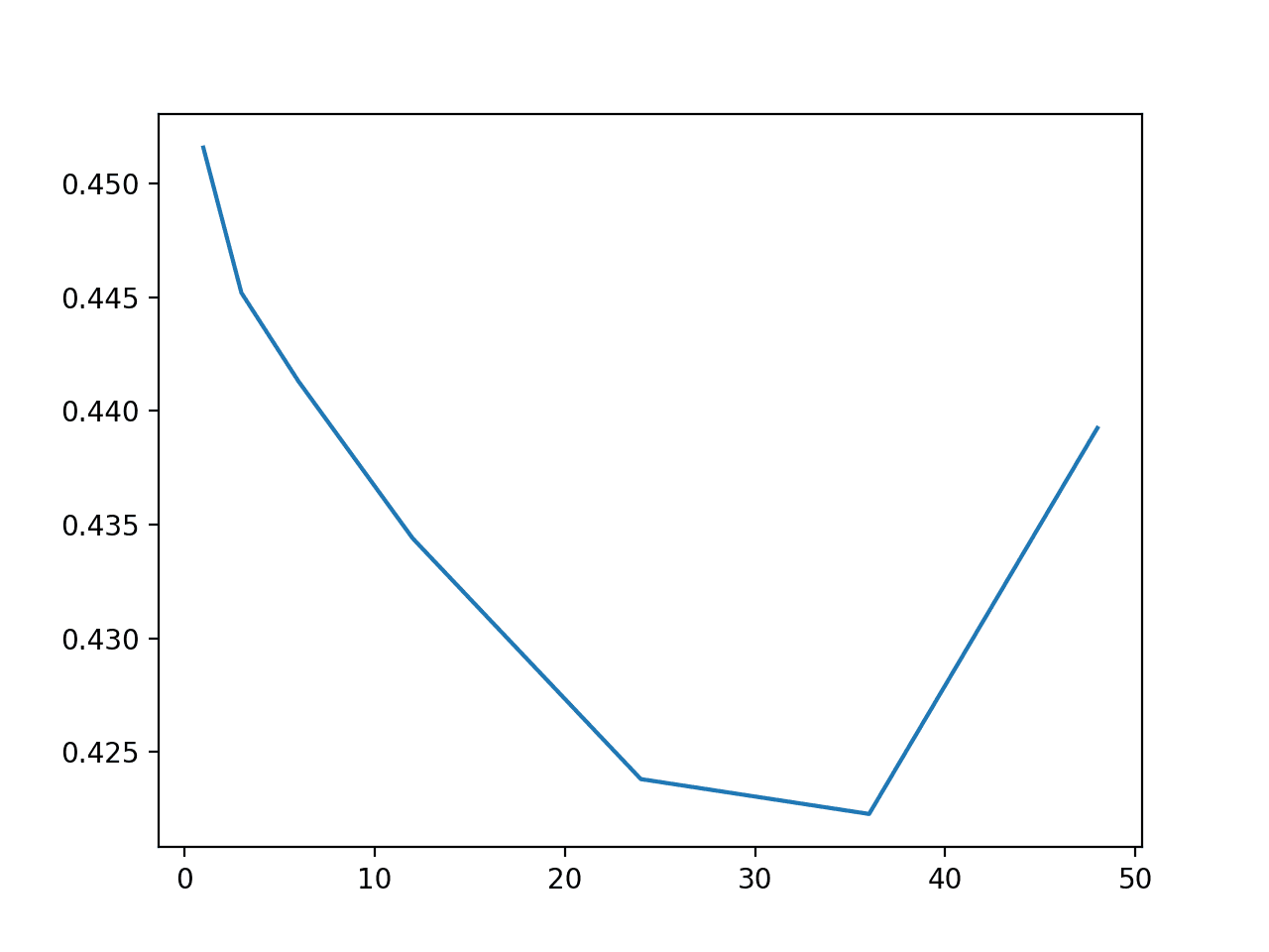
Line Plot of Number of Lag Observations vs MAE for Huber Regression
We can see a general trend of decreasing overall MAE with the increase in the number of lag observations, at least to a point after which error begins to rise again.
The results suggest, at least for the HuberRegressor algorithm, that 36 lag observations may be a good configuration achieving a MAE of 0.422.
Extensions
This section lists some ideas for extending the tutorial that you may wish to explore.
- Data Preparation. Explore whether simple data preparation such as standardization or statistical outlier removal can improve model performance.
- Engineered Features. Explore whether engineered features such as median value for forecasted hour of day can improve model performance
- Meteorological Variables. Explore whether adding lag meteorological variables to the models can improve performance.
- Cross-Site Models. Explore whether combining target variables of the same type and re-using the models across sites results in a performance improvement.
- Algorithm Tuning. Explore whether tuning the hyperparameters of some of the better performing algorithms can result in performance improvements.
If you explore any of these extensions, I’d love to know.
Further Reading
This section provides more resources on the topic if you are looking to go deeper.
- EMC Data Science Global Hackathon (Air Quality Prediction)
- Chucking everything into a Random Forest: Ben Hamner on Winning The Air Quality Prediction Hackathon
- Winning Code for the EMC Data Science Global Hackathon (Air Quality Prediction)
- General approaches to partitioning the models?
Summary
In this tutorial, you discovered how to develop machine learning models for multi-step time series forecasting of air pollution data.
Specifically, you learned:
- How to impute missing values and transform time series data so that it can be modeled by supervised learning algorithms.
- How to develop and evaluate a suite of linear algorithms for multi-step time series forecasting.
- How to develop and evaluate a suite of nonlinear algorithms for multi-step time series forecasting.
Do you have any questions?
Ask your questions in the comments below and I will do my best to answer.
The post How to Develop Machine Learning Models for Multivariate Multi-Step Air Pollution Time Series Forecasting appeared first on Machine Learning Mastery.