
Author: Jason Brownlee
Convolutional Neural Network models, or CNNs for short, can be applied to time series forecasting.
There are many types of CNN models that can be used for each specific type of time series forecasting problem.
In this tutorial, you will discover how to develop a suite of CNN models for a range of standard time series forecasting problems.
The objective of this tutorial is to provide standalone examples of each model on each type of time series problem as a template that you can copy and adapt for your specific time series forecasting problem.
After completing this tutorial, you will know:
- How to develop CNN models for univariate time series forecasting.
- How to develop CNN models for multivariate time series forecasting.
- How to develop CNN models for multi-step time series forecasting.
This is a large and important post; you may want to bookmark it for future reference.
Let’s get started.

How to Develop Convolutional Neural Network Models for Time Series Forecasting
Photo by Bureau of Land Management, some rights reserved.
Tutorial Overview
In this tutorial, we will explore how to develop a suite of different types of CNN models for time series forecasting.
The models are demonstrated on small contrived time series problems intended to give the flavor of the type of time series problem being addressed. The chosen configuration of the models is arbitrary and not optimized for each problem; that was not the goal.
This tutorial is divided into four parts; they are:
- Univariate CNN Models
- Multivariate CNN Models
- Multi-Step CNN Models
- Multivariate Multi-Step CNN Models
Univariate CNN Models
Although traditionally developed for two-dimensional image data, CNNs can be used to model univariate time series forecasting problems.
Univariate time series are datasets comprised of a single series of observations with a temporal ordering and a model is required to learn from the series of past observations to predict the next value in the sequence.
This section is divided into two parts; they are:
- Data Preparation
- CNN Model
Data Preparation
Before a univariate series can be modeled, it must be prepared.
The CNN model will learn a function that maps a sequence of past observations as input to an output observation. As such, the sequence of observations must be transformed into multiple examples from which the model can learn.
Consider a given univariate sequence:
[10, 20, 30, 40, 50, 60, 70, 80, 90]
We can divide the sequence into multiple input/output patterns called samples, where three time steps are used as input and one time step is used as output for the one-step prediction that is being learned.
X,				y
10, 20, 30		40
20, 30, 40		50
30, 40, 50		60
...
The split_sequence() function below implements this behavior and will split a given univariate sequence into multiple samples where each sample has a specified number of time steps and the output is a single time step.
# split a univariate sequence into samples
def split_sequence(sequence, n_steps):
	X, y = list(), list()
	for i in range(len(sequence)):
		# find the end of this pattern
		end_ix = i + n_steps
		# check if we are beyond the sequence
		if end_ix > len(sequence)-1:
			break
		# gather input and output parts of the pattern
		seq_x, seq_y = sequence[i:end_ix], sequence[end_ix]
		X.append(seq_x)
		y.append(seq_y)
	return array(X), array(y)
We can demonstrate this function on our small contrived dataset above.
The complete example is listed below.
# univariate data preparation
from numpy import array

# split a univariate sequence into samples
def split_sequence(sequence, n_steps):
	X, y = list(), list()
	for i in range(len(sequence)):
		# find the end of this pattern
		end_ix = i + n_steps
		# check if we are beyond the sequence
		if end_ix > len(sequence)-1:
			break
		# gather input and output parts of the pattern
		seq_x, seq_y = sequence[i:end_ix], sequence[end_ix]
		X.append(seq_x)
		y.append(seq_y)
	return array(X), array(y)

# define input sequence
raw_seq = [10, 20, 30, 40, 50, 60, 70, 80, 90]
# choose a number of time steps
n_steps = 3
# split into samples
X, y = split_sequence(raw_seq, n_steps)
# summarize the data
for i in range(len(X)):
	print(X[i], y[i])
Running the example splits the univariate series into six samples where each sample has three input time steps and one output time step.
[10 20 30] 40
[20 30 40] 50
[30 40 50] 60
[40 50 60] 70
[50 60 70] 80
[60 70 80] 90
Now that we know how to prepare a univariate series for modeling, let’s look at developing a CNN model that can learn the mapping of inputs to outputs.
Need help with Deep Learning for Time Series?
Take my free 7-day email crash course now (with sample code).
Click to sign-up and also get a free PDF Ebook version of the course.
CNN Model
A one-dimensional CNN is a CNN model that has a convolutional hidden layer that operates over a 1D sequence. This is followed by perhaps a second convolutional layer in some cases, such as very long input sequences, and then a pooling layer whose job it is to distill the output of the convolutional layer to the most salient elements.
The convolutional and pooling layers are followed by a dense fully connected layer that interprets the features extracted by the convolutional part of the model. A flatten layer is used between the convolutional layers and the dense layer to reduce the feature maps to a single one-dimensional vector.
We can define a 1D CNN Model for univariate time series forecasting as follows.
# define model
model = Sequential()
model.add(Conv1D(filters=64, kernel_size=2, activation='relu', input_shape=(n_steps, n_features)))
model.add(MaxPooling1D(pool_size=2))
model.add(Flatten())
model.add(Dense(50, activation='relu'))
model.add(Dense(1))
model.compile(optimizer='adam', loss='mse')
Key in the definition is the shape of the input; that is what the model expects as input for each sample in terms of the number of time steps and the number of features.
We are working with a univariate series, so the number of features is one, for one variable.
The number of time steps as input is the number we chose when preparing our dataset as an argument to the split_sequence() function.
The input shape for each sample is specified in the input_shape argument on the definition of the first hidden layer.
We almost always have multiple samples, therefore, the model will expect the input component of training data to have the dimensions or shape:
[samples, timesteps, features]
Our split_sequence() function in the previous section outputs the X with the shape [samples, timesteps], so we can easily reshape it to have an additional dimension for the one feature.
# reshape from [samples, timesteps] into [samples, timesteps, features]
n_features = 1
X = X.reshape((X.shape[0], X.shape[1], n_features))
The CNN does not actually view the data as having time steps, instead, it is treated as a sequence over which convolutional read operations can be performed, like a one-dimensional image.
In this example, we define a convolutional layer with 64 filter maps and a kernel size of 2. This is followed by a max pooling layer and a dense layer to interpret the input feature. An output layer is specified that predicts a single numerical value.
The model is fit using the efficient Adam version of stochastic gradient descent and optimized using the mean squared error, or ‘mse‘, loss function.
Once the model is defined, we can fit it on the training dataset.
# fit model
model.fit(X, y, epochs=1000, verbose=0)
After the model is fit, we can use it to make a prediction.
We can predict the next value in the sequence by providing the input:
[70, 80, 90]
And expecting the model to predict something like:
[100]
The model expects the input shape to be three-dimensional with [samples, timesteps, features], therefore, we must reshape the single input sample before making the prediction.
# demonstrate prediction
x_input = array([70, 80, 90])
x_input = x_input.reshape((1, n_steps, n_features))
yhat = model.predict(x_input, verbose=0)
We can tie all of this together and demonstrate how to develop a 1D CNN model for univariate time series forecasting and make a single prediction.
# univariate cnn example
from numpy import array
from keras.models import Sequential
from keras.layers import Dense
from keras.layers import Flatten
from keras.layers.convolutional import Conv1D
from keras.layers.convolutional import MaxPooling1D

# split a univariate sequence into samples
def split_sequence(sequence, n_steps):
	X, y = list(), list()
	for i in range(len(sequence)):
		# find the end of this pattern
		end_ix = i + n_steps
		# check if we are beyond the sequence
		if end_ix > len(sequence)-1:
			break
		# gather input and output parts of the pattern
		seq_x, seq_y = sequence[i:end_ix], sequence[end_ix]
		X.append(seq_x)
		y.append(seq_y)
	return array(X), array(y)

# define input sequence
raw_seq = [10, 20, 30, 40, 50, 60, 70, 80, 90]
# choose a number of time steps
n_steps = 3
# split into samples
X, y = split_sequence(raw_seq, n_steps)
# reshape from [samples, timesteps] into [samples, timesteps, features]
n_features = 1
X = X.reshape((X.shape[0], X.shape[1], n_features))
# define model
model = Sequential()
model.add(Conv1D(filters=64, kernel_size=2, activation='relu', input_shape=(n_steps, n_features)))
model.add(MaxPooling1D(pool_size=2))
model.add(Flatten())
model.add(Dense(50, activation='relu'))
model.add(Dense(1))
model.compile(optimizer='adam', loss='mse')
# fit model
model.fit(X, y, epochs=1000, verbose=0)
# demonstrate prediction
x_input = array([70, 80, 90])
x_input = x_input.reshape((1, n_steps, n_features))
yhat = model.predict(x_input, verbose=0)
print(yhat)
Running the example prepares the data, fits the model, and makes a prediction.
Your results may vary given the stochastic nature of the algorithm; try running the example a few times.
We can see that the model predicts the next value in the sequence.
[[101.67965]]
Multivariate CNN Models
Multivariate time series data means data where there is more than one observation for each time step.
There are two main models that we may require with multivariate time series data; they are:
- Multiple Input Series.
- Multiple Parallel Series.
Let’s take a look at each in turn.
Multiple Input Series
A problem may have two or more parallel input time series and an output time series that is dependent on the input time series.
The input time series are parallel because each series has observations at the same time steps.
We can demonstrate this with a simple example of two parallel input time series where the output series is the simple addition of the input series.
# define input sequence
in_seq1 = array([10, 20, 30, 40, 50, 60, 70, 80, 90])
in_seq2 = array([15, 25, 35, 45, 55, 65, 75, 85, 95])
out_seq = array([in_seq1[i]+in_seq2[i] for i in range(len(in_seq1))])
We can reshape these three arrays of data as a single dataset where each row is a time step and each column is a separate time series.
This is a standard way of storing parallel time series in a CSV file.
# convert to [rows, columns] structure
in_seq1 = in_seq1.reshape((len(in_seq1), 1))
in_seq2 = in_seq2.reshape((len(in_seq2), 1))
out_seq = out_seq.reshape((len(out_seq), 1))
# horizontally stack columns
dataset = hstack((in_seq1, in_seq2, out_seq))
The complete example is listed below.
# multivariate data preparation
from numpy import array
from numpy import hstack
# define input sequence
in_seq1 = array([10, 20, 30, 40, 50, 60, 70, 80, 90])
in_seq2 = array([15, 25, 35, 45, 55, 65, 75, 85, 95])
out_seq = array([in_seq1[i]+in_seq2[i] for i in range(len(in_seq1))])
# convert to [rows, columns] structure
in_seq1 = in_seq1.reshape((len(in_seq1), 1))
in_seq2 = in_seq2.reshape((len(in_seq2), 1))
out_seq = out_seq.reshape((len(out_seq), 1))
# horizontally stack columns
dataset = hstack((in_seq1, in_seq2, out_seq))
print(dataset)
Running the example prints the dataset with one row per time step and one column for each of the two input and one output parallel time series.
[[ 10  15  25]
 [ 20  25  45]
 [ 30  35  65]
 [ 40  45  85]
 [ 50  55 105]
 [ 60  65 125]
 [ 70  75 145]
 [ 80  85 165]
 [ 90  95 185]]
As with the univariate time series, we must structure these data into samples with input and output samples.
A 1D CNN model needs sufficient context to learn a mapping from an input sequence to an output value. CNNs can support parallel input time series as separate channels, like red, green, and blue components of an image. Therefore, we need to split the data into samples maintaining the order of observations across the two input sequences.
If we chose three input time steps, then the first sample would look as follows:
Input:
10, 15
20, 25
30, 35
Output:
65
That is, the first three time steps of each parallel series are provided as input to the model and the model associates this with the value in the output series at the third time step, in this case, 65.
We can see that, in transforming the time series into input/output samples to train the model, that we will have to discard some values from the output time series where we do not have values in the input time series at prior time steps. In turn, the choice of the size of the number of input time steps will have an important effect on how much of the training data is used.
We can define a function named split_sequences() that will take a dataset as we have defined it with rows for time steps and columns for parallel series and return input/output samples.
# split a multivariate sequence into samples
def split_sequences(sequences, n_steps):
	X, y = list(), list()
	for i in range(len(sequences)):
		# find the end of this pattern
		end_ix = i + n_steps
		# check if we are beyond the dataset
		if end_ix > len(sequences):
			break
		# gather input and output parts of the pattern
		seq_x, seq_y = sequences[i:end_ix, :-1], sequences[end_ix-1, -1]
		X.append(seq_x)
		y.append(seq_y)
	return array(X), array(y)
We can test this function on our dataset using three time steps for each input time series as input.
The complete example is listed below.
# multivariate data preparation
from numpy import array
from numpy import hstack

# split a multivariate sequence into samples
def split_sequences(sequences, n_steps):
	X, y = list(), list()
	for i in range(len(sequences)):
		# find the end of this pattern
		end_ix = i + n_steps
		# check if we are beyond the dataset
		if end_ix > len(sequences):
			break
		# gather input and output parts of the pattern
		seq_x, seq_y = sequences[i:end_ix, :-1], sequences[end_ix-1, -1]
		X.append(seq_x)
		y.append(seq_y)
	return array(X), array(y)

# define input sequence
in_seq1 = array([10, 20, 30, 40, 50, 60, 70, 80, 90])
in_seq2 = array([15, 25, 35, 45, 55, 65, 75, 85, 95])
out_seq = array([in_seq1[i]+in_seq2[i] for i in range(len(in_seq1))])
# convert to [rows, columns] structure
in_seq1 = in_seq1.reshape((len(in_seq1), 1))
in_seq2 = in_seq2.reshape((len(in_seq2), 1))
out_seq = out_seq.reshape((len(out_seq), 1))
# horizontally stack columns
dataset = hstack((in_seq1, in_seq2, out_seq))
# choose a number of time steps
n_steps = 3
# convert into input/output
X, y = split_sequences(dataset, n_steps)
print(X.shape, y.shape)
# summarize the data
for i in range(len(X)):
	print(X[i], y[i])
Running the example first prints the shape of the X and y components.
We can see that the X component has a three-dimensional structure.
The first dimension is the number of samples, in this case 7. The second dimension is the number of time steps per sample, in this case 3, the value specified to the function. Finally, the last dimension specifies the number of parallel time series or the number of variables, in this case 2 for the two parallel series.
This is the exact three-dimensional structure expected by a 1D CNN as input. The data is ready to use without further reshaping.
We can then see that the input and output for each sample is printed, showing the three time steps for each of the two input series and the associated output for each sample.
(7, 3, 2) (7,)

[[10 15]
 [20 25]
 [30 35]] 65
[[20 25]
 [30 35]
 [40 45]] 85
[[30 35]
 [40 45]
 [50 55]] 105
[[40 45]
 [50 55]
 [60 65]] 125
[[50 55]
 [60 65]
 [70 75]] 145
[[60 65]
 [70 75]
 [80 85]] 165
[[70 75]
 [80 85]
 [90 95]] 185
We are now ready to fit a 1D CNN model on this data, specifying the expected number of time steps and features to expect for each input sample, in this case three and two respectively.
# define model
model = Sequential()
model.add(Conv1D(filters=64, kernel_size=2, activation='relu', input_shape=(n_steps, n_features)))
model.add(MaxPooling1D(pool_size=2))
model.add(Flatten())
model.add(Dense(50, activation='relu'))
model.add(Dense(1))
model.compile(optimizer='adam', loss='mse')
When making a prediction, the model expects three time steps for two input time series.
We can predict the next value in the output series providing the input values of:
80,	 85
90,	 95
100, 105
The shape of the one sample with three time steps and two variables must be [1, 3, 2].
We would expect the next value in the sequence to be 100 + 105 or 205.
# demonstrate prediction
x_input = array([[80, 85], [90, 95], [100, 105]])
x_input = x_input.reshape((1, n_steps, n_features))
yhat = model.predict(x_input, verbose=0)
The complete example is listed below.
# multivariate cnn example
from numpy import array
from numpy import hstack
from keras.models import Sequential
from keras.layers import Dense
from keras.layers import Flatten
from keras.layers.convolutional import Conv1D
from keras.layers.convolutional import MaxPooling1D

# split a multivariate sequence into samples
def split_sequences(sequences, n_steps):
	X, y = list(), list()
	for i in range(len(sequences)):
		# find the end of this pattern
		end_ix = i + n_steps
		# check if we are beyond the dataset
		if end_ix > len(sequences):
			break
		# gather input and output parts of the pattern
		seq_x, seq_y = sequences[i:end_ix, :-1], sequences[end_ix-1, -1]
		X.append(seq_x)
		y.append(seq_y)
	return array(X), array(y)

# define input sequence
in_seq1 = array([10, 20, 30, 40, 50, 60, 70, 80, 90])
in_seq2 = array([15, 25, 35, 45, 55, 65, 75, 85, 95])
out_seq = array([in_seq1[i]+in_seq2[i] for i in range(len(in_seq1))])
# convert to [rows, columns] structure
in_seq1 = in_seq1.reshape((len(in_seq1), 1))
in_seq2 = in_seq2.reshape((len(in_seq2), 1))
out_seq = out_seq.reshape((len(out_seq), 1))
# horizontally stack columns
dataset = hstack((in_seq1, in_seq2, out_seq))
# choose a number of time steps
n_steps = 3
# convert into input/output
X, y = split_sequences(dataset, n_steps)
# the dataset knows the number of features, e.g. 2
n_features = X.shape[2]
# define model
model = Sequential()
model.add(Conv1D(filters=64, kernel_size=2, activation='relu', input_shape=(n_steps, n_features)))
model.add(MaxPooling1D(pool_size=2))
model.add(Flatten())
model.add(Dense(50, activation='relu'))
model.add(Dense(1))
model.compile(optimizer='adam', loss='mse')
# fit model
model.fit(X, y, epochs=1000, verbose=0)
# demonstrate prediction
x_input = array([[80, 85], [90, 95], [100, 105]])
x_input = x_input.reshape((1, n_steps, n_features))
yhat = model.predict(x_input, verbose=0)
print(yhat)
Running the example prepares the data, fits the model, and makes a prediction.
[[206.0161]]
There is another, more elaborate way to model the problem.
Each input series can be handled by a separate CNN and the output of each of these submodels can be combined before a prediction is made for the output sequence.
We can refer to this as a multi-headed CNN model. It may offer more flexibility or better performance depending on the specifics of the problem that is being modeled. For example, it allows you to configure each sub-model differently for each input series, such as the number of filter maps and the kernel size.
This type of model can be defined in Keras using the Keras functional API.
First, we can define the first input model as a 1D CNN with an input layer that expects vectors with n_steps and 1 feature.
# first input model
visible1 = Input(shape=(n_steps, n_features))
cnn1 = Conv1D(filters=64, kernel_size=2, activation='relu')(visible1)
cnn1 = MaxPooling1D(pool_size=2)(cnn1)
cnn1 = Flatten()(cnn1)
We can define the second input submodel in the same way.
# second input model
visible2 = Input(shape=(n_steps, n_features))
cnn2 = Conv1D(filters=64, kernel_size=2, activation='relu')(visible2)
cnn2 = MaxPooling1D(pool_size=2)(cnn2)
cnn2 = Flatten()(cnn2)
Now that both input submodels have been defined, we can merge the output from each model into one long vector which can be interpreted before making a prediction for the output sequence.
# merge input models
merge = concatenate([cnn1, cnn2])
dense = Dense(50, activation='relu')(merge)
output = Dense(1)(dense)
We can then tie the inputs and outputs together.
model = Model(inputs=[visible1, visible2], outputs=output)
The image below provides a schematic for how this model looks, including the shape of the inputs and outputs of each layer.
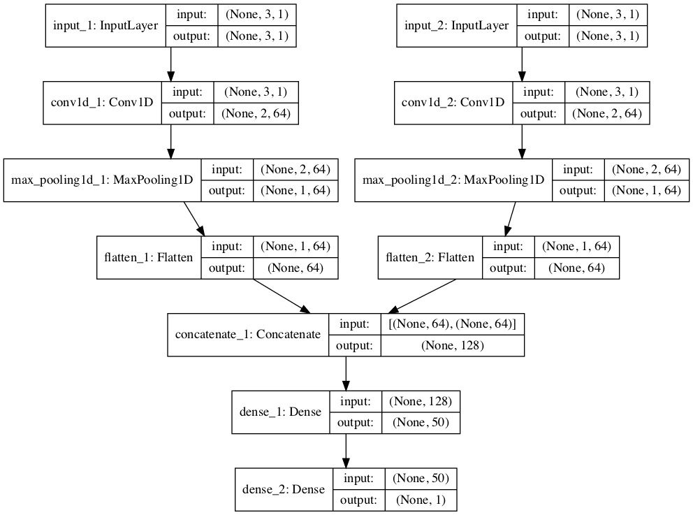
Plot of Multi-Headed 1D CNN for Multivariate Time Series Forecasting
This model requires input to be provided as a list of two elements where each element in the list contains data for one of the submodels.
In order to achieve this, we can split the 3D input data into two separate arrays of input data; that is from one array with the shape [7, 3, 2] to two 3D arrays with [7, 3, 1]
# one time series per head
n_features = 1
# separate input data
X1 = X[:, :, 0].reshape(X.shape[0], X.shape[1], n_features)
X2 = X[:, :, 1].reshape(X.shape[0], X.shape[1], n_features)
These data can then be provided in order to fit the model.
# fit model
model.fit([X1, X2], y, epochs=1000, verbose=0)
Similarly, we must prepare the data for a single sample as two separate two-dimensional arrays when making a single one-step prediction.
x_input = array([[80, 85], [90, 95], [100, 105]])
x1 = x_input[:, 0].reshape((1, n_steps, n_features))
x2 = x_input[:, 1].reshape((1, n_steps, n_features))
We can tie all of this together; the complete example is listed below.
# multivariate multi-headed 1d cnn example
from numpy import array
from numpy import hstack
from keras.models import Model
from keras.layers import Input
from keras.layers import Dense
from keras.layers import Flatten
from keras.layers.convolutional import Conv1D
from keras.layers.convolutional import MaxPooling1D
from keras.layers.merge import concatenate

# split a multivariate sequence into samples
def split_sequences(sequences, n_steps):
	X, y = list(), list()
	for i in range(len(sequences)):
		# find the end of this pattern
		end_ix = i + n_steps
		# check if we are beyond the dataset
		if end_ix > len(sequences):
			break
		# gather input and output parts of the pattern
		seq_x, seq_y = sequences[i:end_ix, :-1], sequences[end_ix-1, -1]
		X.append(seq_x)
		y.append(seq_y)
	return array(X), array(y)

# define input sequence
in_seq1 = array([10, 20, 30, 40, 50, 60, 70, 80, 90])
in_seq2 = array([15, 25, 35, 45, 55, 65, 75, 85, 95])
out_seq = array([in_seq1[i]+in_seq2[i] for i in range(len(in_seq1))])
# convert to [rows, columns] structure
in_seq1 = in_seq1.reshape((len(in_seq1), 1))
in_seq2 = in_seq2.reshape((len(in_seq2), 1))
out_seq = out_seq.reshape((len(out_seq), 1))
# horizontally stack columns
dataset = hstack((in_seq1, in_seq2, out_seq))
# choose a number of time steps
n_steps = 3
# convert into input/output
X, y = split_sequences(dataset, n_steps)
# one time series per head
n_features = 1
# separate input data
X1 = X[:, :, 0].reshape(X.shape[0], X.shape[1], n_features)
X2 = X[:, :, 1].reshape(X.shape[0], X.shape[1], n_features)
# first input model
visible1 = Input(shape=(n_steps, n_features))
cnn1 = Conv1D(filters=64, kernel_size=2, activation='relu')(visible1)
cnn1 = MaxPooling1D(pool_size=2)(cnn1)
cnn1 = Flatten()(cnn1)
# second input model
visible2 = Input(shape=(n_steps, n_features))
cnn2 = Conv1D(filters=64, kernel_size=2, activation='relu')(visible2)
cnn2 = MaxPooling1D(pool_size=2)(cnn2)
cnn2 = Flatten()(cnn2)
# merge input models
merge = concatenate([cnn1, cnn2])
dense = Dense(50, activation='relu')(merge)
output = Dense(1)(dense)
model = Model(inputs=[visible1, visible2], outputs=output)
model.compile(optimizer='adam', loss='mse')
# fit model
model.fit([X1, X2], y, epochs=1000, verbose=0)
# demonstrate prediction
x_input = array([[80, 85], [90, 95], [100, 105]])
x1 = x_input[:, 0].reshape((1, n_steps, n_features))
x2 = x_input[:, 1].reshape((1, n_steps, n_features))
yhat = model.predict([x1, x2], verbose=0)
print(yhat)
Running the example prepares the data, fits the model, and makes a prediction.
[[205.871]]
Multiple Parallel Series
An alternate time series problem is the case where there are multiple parallel time series and a value must be predicted for each.
For example, given the data from the previous section:
[[ 10  15  25]
 [ 20  25  45]
 [ 30  35  65]
 [ 40  45  85]
 [ 50  55 105]
 [ 60  65 125]
 [ 70  75 145]
 [ 80  85 165]
 [ 90  95 185]]
We may want to predict the value for each of the three time series for the next time step.
This might be referred to as multivariate forecasting.
Again, the data must be split into input/output samples in order to train a model.
The first sample of this dataset would be:
Input:
10, 15, 25
20, 25, 45
30, 35, 65
Output:
40, 45, 85
The split_sequences() function below will split multiple parallel time series with rows for time steps and one series per column into the required input/output shape.
# split a multivariate sequence into samples
def split_sequences(sequences, n_steps):
	X, y = list(), list()
	for i in range(len(sequences)):
		# find the end of this pattern
		end_ix = i + n_steps
		# check if we are beyond the dataset
		if end_ix > len(sequences)-1:
			break
		# gather input and output parts of the pattern
		seq_x, seq_y = sequences[i:end_ix, :], sequences[end_ix, :]
		X.append(seq_x)
		y.append(seq_y)
	return array(X), array(y)
We can demonstrate this on the contrived problem; the complete example is listed below.
# multivariate output data prep
from numpy import array
from numpy import hstack

# split a multivariate sequence into samples
def split_sequences(sequences, n_steps):
	X, y = list(), list()
	for i in range(len(sequences)):
		# find the end of this pattern
		end_ix = i + n_steps
		# check if we are beyond the dataset
		if end_ix > len(sequences)-1:
			break
		# gather input and output parts of the pattern
		seq_x, seq_y = sequences[i:end_ix, :], sequences[end_ix, :]
		X.append(seq_x)
		y.append(seq_y)
	return array(X), array(y)

# define input sequence
in_seq1 = array([10, 20, 30, 40, 50, 60, 70, 80, 90])
in_seq2 = array([15, 25, 35, 45, 55, 65, 75, 85, 95])
out_seq = array([in_seq1[i]+in_seq2[i] for i in range(len(in_seq1))])
# convert to [rows, columns] structure
in_seq1 = in_seq1.reshape((len(in_seq1), 1))
in_seq2 = in_seq2.reshape((len(in_seq2), 1))
out_seq = out_seq.reshape((len(out_seq), 1))
# horizontally stack columns
dataset = hstack((in_seq1, in_seq2, out_seq))
# choose a number of time steps
n_steps = 3
# convert into input/output
X, y = split_sequences(dataset, n_steps)
print(X.shape, y.shape)
# summarize the data
for i in range(len(X)):
	print(X[i], y[i])
Running the example first prints the shape of the prepared X and y components.
The shape of X is three-dimensional, including the number of samples (6), the number of time steps chosen per sample (3), and the number of parallel time series or features (3).
The shape of y is two-dimensional as we might expect for the number of samples (6) and the number of time variables per sample to be predicted (3).
The data is ready to use in a 1D CNN model that expects three-dimensional input and two-dimensional output shapes for the X and y components of each sample.
Then, each of the samples is printed showing the input and output components of each sample.
(6, 3, 3) (6, 3)

[[10 15 25]
 [20 25 45]
 [30 35 65]] [40 45 85]
[[20 25 45]
 [30 35 65]
 [40 45 85]] [ 50  55 105]
[[ 30  35  65]
 [ 40  45  85]
 [ 50  55 105]] [ 60  65 125]
[[ 40  45  85]
 [ 50  55 105]
 [ 60  65 125]] [ 70  75 145]
[[ 50  55 105]
 [ 60  65 125]
 [ 70  75 145]] [ 80  85 165]
[[ 60  65 125]
 [ 70  75 145]
 [ 80  85 165]] [ 90  95 185]
We are now ready to fit a 1D CNN model on this data.
In this model, the number of time steps and parallel series (features) are specified for the input layer via the input_shape argument.
The number of parallel series is also used in the specification of the number of values to predict by the model in the output layer; again, this is three.
# define model
model = Sequential()
model.add(Conv1D(filters=64, kernel_size=2, activation='relu', input_shape=(n_steps, n_features)))
model.add(MaxPooling1D(pool_size=2))
model.add(Flatten())
model.add(Dense(50, activation='relu'))
model.add(Dense(n_features))
model.compile(optimizer='adam', loss='mse')
We can predict the next value in each of the three parallel series by providing an input of three time steps for each series.
70, 75, 145
80, 85, 165
90, 95, 185
The shape of the input for making a single prediction must be 1 sample, 3 time steps, and 3 features, or [1, 3, 3].
# demonstrate prediction
x_input = array([[70,75,145], [80,85,165], [90,95,185]])
x_input = x_input.reshape((1, n_steps, n_features))
yhat = model.predict(x_input, verbose=0)
We would expect the vector output to be:
[100, 105, 205]
We can tie all of this together and demonstrate a 1D CNN for multivariate output time series forecasting below.
# multivariate output 1d cnn example
from numpy import array
from numpy import hstack
from keras.models import Sequential
from keras.layers import Dense
from keras.layers import Flatten
from keras.layers.convolutional import Conv1D
from keras.layers.convolutional import MaxPooling1D

# split a multivariate sequence into samples
def split_sequences(sequences, n_steps):
	X, y = list(), list()
	for i in range(len(sequences)):
		# find the end of this pattern
		end_ix = i + n_steps
		# check if we are beyond the dataset
		if end_ix > len(sequences)-1:
			break
		# gather input and output parts of the pattern
		seq_x, seq_y = sequences[i:end_ix, :], sequences[end_ix, :]
		X.append(seq_x)
		y.append(seq_y)
	return array(X), array(y)

# define input sequence
in_seq1 = array([10, 20, 30, 40, 50, 60, 70, 80, 90])
in_seq2 = array([15, 25, 35, 45, 55, 65, 75, 85, 95])
out_seq = array([in_seq1[i]+in_seq2[i] for i in range(len(in_seq1))])
# convert to [rows, columns] structure
in_seq1 = in_seq1.reshape((len(in_seq1), 1))
in_seq2 = in_seq2.reshape((len(in_seq2), 1))
out_seq = out_seq.reshape((len(out_seq), 1))
# horizontally stack columns
dataset = hstack((in_seq1, in_seq2, out_seq))
# choose a number of time steps
n_steps = 3
# convert into input/output
X, y = split_sequences(dataset, n_steps)
# the dataset knows the number of features, e.g. 2
n_features = X.shape[2]
# define model
model = Sequential()
model.add(Conv1D(filters=64, kernel_size=2, activation='relu', input_shape=(n_steps, n_features)))
model.add(MaxPooling1D(pool_size=2))
model.add(Flatten())
model.add(Dense(50, activation='relu'))
model.add(Dense(n_features))
model.compile(optimizer='adam', loss='mse')
# fit model
model.fit(X, y, epochs=3000, verbose=0)
# demonstrate prediction
x_input = array([[70,75,145], [80,85,165], [90,95,185]])
x_input = x_input.reshape((1, n_steps, n_features))
yhat = model.predict(x_input, verbose=0)
print(yhat)
Running the example prepares the data, fits the model and makes a prediction.
[[100.11272 105.32213 205.53436]]
As with multiple input series, there is another more elaborate way to model the problem.
Each output series can be handled by a separate output CNN model.
We can refer to this as a multi-output CNN model. It may offer more flexibility or better performance depending on the specifics of the problem that is being modeled.
This type of model can be defined in Keras using the Keras functional API.
First, we can define the first input model as a 1D CNN model.
# define model
visible = Input(shape=(n_steps, n_features))
cnn = Conv1D(filters=64, kernel_size=2, activation='relu')(visible)
cnn = MaxPooling1D(pool_size=2)(cnn)
cnn = Flatten()(cnn)
cnn = Dense(50, activation='relu')(cnn)
We can then define one output layer for each of the three series that we wish to forecast, where each output submodel will forecast a single time step.
# define output 1
output1 = Dense(1)(cnn)
# define output 2
output2 = Dense(1)(cnn)
# define output 3
output3 = Dense(1)(cnn)
We can then tie the input and output layers together into a single model.
# tie together
model = Model(inputs=visible, outputs=[output1, output2, output3])
model.compile(optimizer='adam', loss='mse')
To make the model architecture clear, the schematic below clearly shows the three separate output layers of the model and the input and output shapes of each layer.
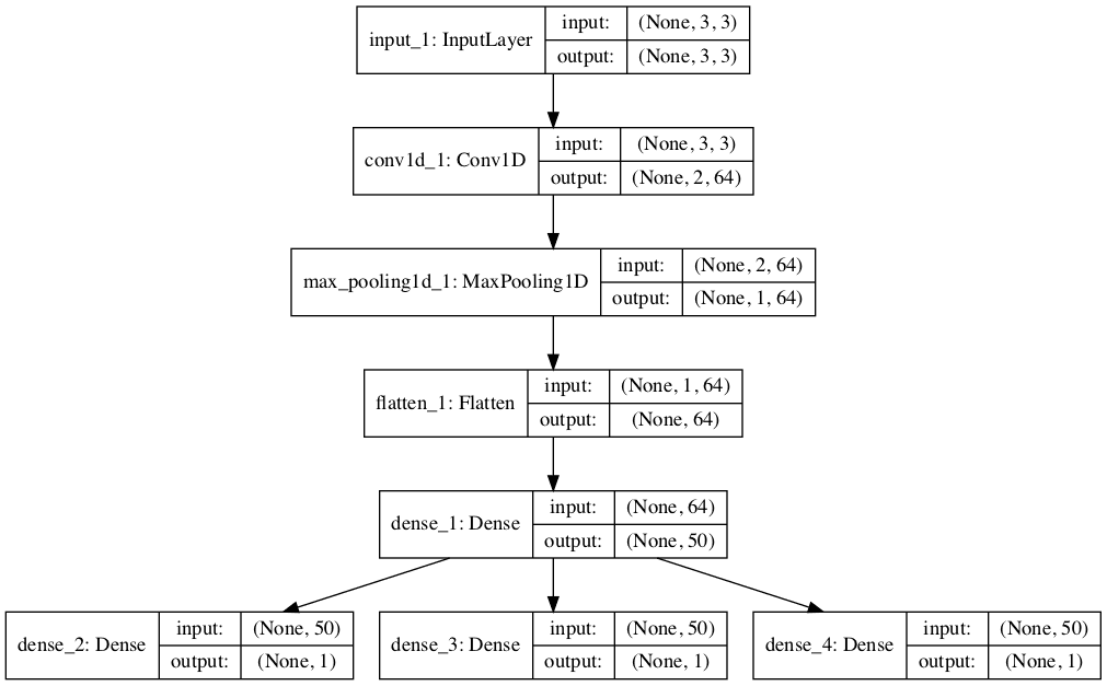
Plot of Multi-Output 1D CNN for Multivariate Time Series Forecasting
When training the model, it will require three separate output arrays per sample. We can achieve this by converting the output training data that has the shape [7, 3] to three arrays with the shape [7, 1].
# separate output
y1 = y[:, 0].reshape((y.shape[0], 1))
y2 = y[:, 1].reshape((y.shape[0], 1))
y3 = y[:, 2].reshape((y.shape[0], 1))
These arrays can be provided to the model during training.
# fit model
model.fit(X, [y1,y2,y3], epochs=2000, verbose=0)
Tying all of this together, the complete example is listed below.
# multivariate output 1d cnn example
from numpy import array
from numpy import hstack
from keras.models import Model
from keras.layers import Input
from keras.layers import Dense
from keras.layers import Flatten
from keras.layers.convolutional import Conv1D
from keras.layers.convolutional import MaxPooling1D

# split a multivariate sequence into samples
def split_sequences(sequences, n_steps):
	X, y = list(), list()
	for i in range(len(sequences)):
		# find the end of this pattern
		end_ix = i + n_steps
		# check if we are beyond the dataset
		if end_ix > len(sequences)-1:
			break
		# gather input and output parts of the pattern
		seq_x, seq_y = sequences[i:end_ix, :], sequences[end_ix, :]
		X.append(seq_x)
		y.append(seq_y)
	return array(X), array(y)

# define input sequence
in_seq1 = array([10, 20, 30, 40, 50, 60, 70, 80, 90])
in_seq2 = array([15, 25, 35, 45, 55, 65, 75, 85, 95])
out_seq = array([in_seq1[i]+in_seq2[i] for i in range(len(in_seq1))])
# convert to [rows, columns] structure
in_seq1 = in_seq1.reshape((len(in_seq1), 1))
in_seq2 = in_seq2.reshape((len(in_seq2), 1))
out_seq = out_seq.reshape((len(out_seq), 1))
# horizontally stack columns
dataset = hstack((in_seq1, in_seq2, out_seq))
# choose a number of time steps
n_steps = 3
# convert into input/output
X, y = split_sequences(dataset, n_steps)
# the dataset knows the number of features, e.g. 2
n_features = X.shape[2]
# separate output
y1 = y[:, 0].reshape((y.shape[0], 1))
y2 = y[:, 1].reshape((y.shape[0], 1))
y3 = y[:, 2].reshape((y.shape[0], 1))
# define model
visible = Input(shape=(n_steps, n_features))
cnn = Conv1D(filters=64, kernel_size=2, activation='relu')(visible)
cnn = MaxPooling1D(pool_size=2)(cnn)
cnn = Flatten()(cnn)
cnn = Dense(50, activation='relu')(cnn)
# define output 1
output1 = Dense(1)(cnn)
# define output 2
output2 = Dense(1)(cnn)
# define output 3
output3 = Dense(1)(cnn)
# tie together
model = Model(inputs=visible, outputs=[output1, output2, output3])
model.compile(optimizer='adam', loss='mse')
# fit model
model.fit(X, [y1,y2,y3], epochs=2000, verbose=0)
# demonstrate prediction
x_input = array([[70,75,145], [80,85,165], [90,95,185]])
x_input = x_input.reshape((1, n_steps, n_features))
yhat = model.predict(x_input, verbose=0)
print(yhat)
Running the example prepares the data, fits the model, and makes a prediction.
[array([[100.96118]], dtype=float32),
 array([[105.502686]], dtype=float32),
 array([[205.98045]], dtype=float32)]
Multi-Step CNN Models
In practice, there is little difference to the 1D CNN model in predicting a vector output that represents different output variables (as in the previous example), or a vector output that represents multiple time steps of one variable.
Nevertheless, there are subtle and important differences in the way the training data is prepared. In this section, we will demonstrate the case of developing a multi-step forecast model using a vector model.
Before we look at the specifics of the model, let’s first look at the preparation of data for multi-step forecasting.
Data Preparation
As with one-step forecasting, a time series used for multi-step time series forecasting must be split into samples with input and output components.
Both the input and output components will be comprised of multiple time steps and may or may not have the same number of steps.
For example, given the univariate time series:
[10, 20, 30, 40, 50, 60, 70, 80, 90]
We could use the last three time steps as input and forecast the next two time steps.
The first sample would look as follows:
Input:
[10, 20, 30]
Output:
[40, 50]
The split_sequence() function below implements this behavior and will split a given univariate time series into samples with a specified number of input and output time steps.
# split a univariate sequence into samples
def split_sequence(sequence, n_steps_in, n_steps_out):
	X, y = list(), list()
	for i in range(len(sequence)):
		# find the end of this pattern
		end_ix = i + n_steps_in
		out_end_ix = end_ix + n_steps_out
		# check if we are beyond the sequence
		if out_end_ix > len(sequence):
			break
		# gather input and output parts of the pattern
		seq_x, seq_y = sequence[i:end_ix], sequence[end_ix:out_end_ix]
		X.append(seq_x)
		y.append(seq_y)
	return array(X), array(y)
We can demonstrate this function on the small contrived dataset.
The complete example is listed below.
# multi-step data preparation
from numpy import array

# split a univariate sequence into samples
def split_sequence(sequence, n_steps_in, n_steps_out):
	X, y = list(), list()
	for i in range(len(sequence)):
		# find the end of this pattern
		end_ix = i + n_steps_in
		out_end_ix = end_ix + n_steps_out
		# check if we are beyond the sequence
		if out_end_ix > len(sequence):
			break
		# gather input and output parts of the pattern
		seq_x, seq_y = sequence[i:end_ix], sequence[end_ix:out_end_ix]
		X.append(seq_x)
		y.append(seq_y)
	return array(X), array(y)

# define input sequence
raw_seq = [10, 20, 30, 40, 50, 60, 70, 80, 90]
# choose a number of time steps
n_steps_in, n_steps_out = 3, 2
# split into samples
X, y = split_sequence(raw_seq, n_steps_in, n_steps_out)
# summarize the data
for i in range(len(X)):
	print(X[i], y[i])
Running the example splits the univariate series into input and output time steps and prints the input and output components of each.
[10 20 30] [40 50]
[20 30 40] [50 60]
[30 40 50] [60 70]
[40 50 60] [70 80]
[50 60 70] [80 90]
Now that we know how to prepare data for multi-step forecasting, let’s look at a 1D CNN model that can learn this mapping.
Vector Output Model
The 1D CNN can output a vector directly that can be interpreted as a multi-step forecast.
This approach was seen in the previous section were one time step of each output time series was forecasted as a vector.
As with the 1D CNN models for univariate data in a prior section, the prepared samples must first be reshaped. The CNN expects data to have a three-dimensional structure of [samples, timesteps, features], and in this case, we only have one feature so the reshape is straightforward.
# reshape from [samples, timesteps] into [samples, timesteps, features]
n_features = 1
X = X.reshape((X.shape[0], X.shape[1], n_features))
With the number of input and output steps specified in the n_steps_in and n_steps_out variables, we can define a multi-step time-series forecasting model.
# define model
model = Sequential()
model.add(Conv1D(filters=64, kernel_size=2, activation='relu', input_shape=(n_steps_in, n_features)))
model.add(MaxPooling1D(pool_size=2))
model.add(Flatten())
model.add(Dense(50, activation='relu'))
model.add(Dense(n_steps_out))
model.compile(optimizer='adam', loss='mse')
The model can make a prediction for a single sample. We can predict the next two steps beyond the end of the dataset by providing the input:
[70, 80, 90]
We would expect the predicted output to be:
[100, 110]
As expected by the model, the shape of the single sample of input data when making the prediction must be [1, 3, 1] for the 1 sample, 3 time steps of the input, and the single feature.
# demonstrate prediction
x_input = array([70, 80, 90])
x_input = x_input.reshape((1, n_steps_in, n_features))
yhat = model.predict(x_input, verbose=0)
Tying all of this together, the 1D CNN for multi-step forecasting with a univariate time series is listed below.
# univariate multi-step vector-output 1d cnn example
from numpy import array
from keras.models import Sequential
from keras.layers import Dense
from keras.layers import Flatten
from keras.layers.convolutional import Conv1D
from keras.layers.convolutional import MaxPooling1D

# split a univariate sequence into samples
def split_sequence(sequence, n_steps_in, n_steps_out):
	X, y = list(), list()
	for i in range(len(sequence)):
		# find the end of this pattern
		end_ix = i + n_steps_in
		out_end_ix = end_ix + n_steps_out
		# check if we are beyond the sequence
		if out_end_ix > len(sequence):
			break
		# gather input and output parts of the pattern
		seq_x, seq_y = sequence[i:end_ix], sequence[end_ix:out_end_ix]
		X.append(seq_x)
		y.append(seq_y)
	return array(X), array(y)

# define input sequence
raw_seq = [10, 20, 30, 40, 50, 60, 70, 80, 90]
# choose a number of time steps
n_steps_in, n_steps_out = 3, 2
# split into samples
X, y = split_sequence(raw_seq, n_steps_in, n_steps_out)
# reshape from [samples, timesteps] into [samples, timesteps, features]
n_features = 1
X = X.reshape((X.shape[0], X.shape[1], n_features))
# define model
model = Sequential()
model.add(Conv1D(filters=64, kernel_size=2, activation='relu', input_shape=(n_steps_in, n_features)))
model.add(MaxPooling1D(pool_size=2))
model.add(Flatten())
model.add(Dense(50, activation='relu'))
model.add(Dense(n_steps_out))
model.compile(optimizer='adam', loss='mse')
# fit model
model.fit(X, y, epochs=2000, verbose=0)
# demonstrate prediction
x_input = array([70, 80, 90])
x_input = x_input.reshape((1, n_steps_in, n_features))
yhat = model.predict(x_input, verbose=0)
print(yhat)
Running the example forecasts and prints the next two time steps in the sequence.
[[102.86651 115.08979]]
Multivariate Multi-Step CNN Models
In the previous sections, we have looked at univariate, multivariate, and multi-step time series forecasting.
It is possible to mix and match the different types of 1D CNN models presented so far for the different problems. This too applies to time series forecasting problems that involve multivariate and multi-step forecasting, but it may be a little more challenging.
In this section, we will explore short examples of data preparation and modeling for multivariate multi-step time series forecasting as a template to ease this challenge, specifically:
- Multiple Input Multi-Step Output.
- Multiple Parallel Input and Multi-Step Output.
Perhaps the biggest stumbling block is in the preparation of data, so this is where we will focus our attention.
Multiple Input Multi-Step Output
There are those multivariate time series forecasting problems where the output series is separate but dependent upon the input time series, and multiple time steps are required for the output series.
For example, consider our multivariate time series from a prior section:
[[ 10  15  25]
 [ 20  25  45]
 [ 30  35  65]
 [ 40  45  85]
 [ 50  55 105]
 [ 60  65 125]
 [ 70  75 145]
 [ 80  85 165]
 [ 90  95 185]]
We may use three prior time steps of each of the two input time series to predict two time steps of the output time series.
Input:
10, 15
20, 25
30, 35
Output:
65
85
The split_sequences() function below implements this behavior.
# split a multivariate sequence into samples
def split_sequences(sequences, n_steps_in, n_steps_out):
	X, y = list(), list()
	for i in range(len(sequences)):
		# find the end of this pattern
		end_ix = i + n_steps_in
		out_end_ix = end_ix + n_steps_out-1
		# check if we are beyond the dataset
		if out_end_ix > len(sequences):
			break
		# gather input and output parts of the pattern
		seq_x, seq_y = sequences[i:end_ix, :-1], sequences[end_ix-1:out_end_ix, -1]
		X.append(seq_x)
		y.append(seq_y)
	return array(X), array(y)
We can demonstrate this on our contrived dataset. The complete example is listed below.
# multivariate multi-step data preparation
from numpy import array
from numpy import hstack

# split a multivariate sequence into samples
def split_sequences(sequences, n_steps_in, n_steps_out):
	X, y = list(), list()
	for i in range(len(sequences)):
		# find the end of this pattern
		end_ix = i + n_steps_in
		out_end_ix = end_ix + n_steps_out-1
		# check if we are beyond the dataset
		if out_end_ix > len(sequences):
			break
		# gather input and output parts of the pattern
		seq_x, seq_y = sequences[i:end_ix, :-1], sequences[end_ix-1:out_end_ix, -1]
		X.append(seq_x)
		y.append(seq_y)
	return array(X), array(y)

# define input sequence
in_seq1 = array([10, 20, 30, 40, 50, 60, 70, 80, 90])
in_seq2 = array([15, 25, 35, 45, 55, 65, 75, 85, 95])
out_seq = array([in_seq1[i]+in_seq2[i] for i in range(len(in_seq1))])
# convert to [rows, columns] structure
in_seq1 = in_seq1.reshape((len(in_seq1), 1))
in_seq2 = in_seq2.reshape((len(in_seq2), 1))
out_seq = out_seq.reshape((len(out_seq), 1))
# horizontally stack columns
dataset = hstack((in_seq1, in_seq2, out_seq))
# choose a number of time steps
n_steps_in, n_steps_out = 3, 2
# convert into input/output
X, y = split_sequences(dataset, n_steps_in, n_steps_out)
print(X.shape, y.shape)
# summarize the data
for i in range(len(X)):
	print(X[i], y[i])
Running the example first prints the shape of the prepared training data.
We can see that the shape of the input portion of the samples is three-dimensional, comprised of six samples, with three time steps and two variables for the two input time series.
The output portion of the samples is two-dimensional for the six samples and the two time steps for each sample to be predicted.
The prepared samples are then printed to confirm that the data was prepared as we specified.
(6, 3, 2) (6, 2)

[[10 15]
 [20 25]
 [30 35]] [65 85]
[[20 25]
 [30 35]
 [40 45]] [ 85 105]
[[30 35]
 [40 45]
 [50 55]] [105 125]
[[40 45]
 [50 55]
 [60 65]] [125 145]
[[50 55]
 [60 65]
 [70 75]] [145 165]
[[60 65]
 [70 75]
 [80 85]] [165 185]
We can now develop a 1D CNN model for multi-step predictions.
In this case, we will demonstrate a vector output model. The complete example is listed below.
# multivariate multi-step 1d cnn example
from numpy import array
from numpy import hstack
from keras.models import Sequential
from keras.layers import Dense
from keras.layers import Flatten
from keras.layers.convolutional import Conv1D
from keras.layers.convolutional import MaxPooling1D

# split a multivariate sequence into samples
def split_sequences(sequences, n_steps_in, n_steps_out):
	X, y = list(), list()
	for i in range(len(sequences)):
		# find the end of this pattern
		end_ix = i + n_steps_in
		out_end_ix = end_ix + n_steps_out-1
		# check if we are beyond the dataset
		if out_end_ix > len(sequences):
			break
		# gather input and output parts of the pattern
		seq_x, seq_y = sequences[i:end_ix, :-1], sequences[end_ix-1:out_end_ix, -1]
		X.append(seq_x)
		y.append(seq_y)
	return array(X), array(y)

# define input sequence
in_seq1 = array([10, 20, 30, 40, 50, 60, 70, 80, 90])
in_seq2 = array([15, 25, 35, 45, 55, 65, 75, 85, 95])
out_seq = array([in_seq1[i]+in_seq2[i] for i in range(len(in_seq1))])
# convert to [rows, columns] structure
in_seq1 = in_seq1.reshape((len(in_seq1), 1))
in_seq2 = in_seq2.reshape((len(in_seq2), 1))
out_seq = out_seq.reshape((len(out_seq), 1))
# horizontally stack columns
dataset = hstack((in_seq1, in_seq2, out_seq))
# choose a number of time steps
n_steps_in, n_steps_out = 3, 2
# convert into input/output
X, y = split_sequences(dataset, n_steps_in, n_steps_out)
# the dataset knows the number of features, e.g. 2
n_features = X.shape[2]
# define model
model = Sequential()
model.add(Conv1D(filters=64, kernel_size=2, activation='relu', input_shape=(n_steps_in, n_features)))
model.add(MaxPooling1D(pool_size=2))
model.add(Flatten())
model.add(Dense(50, activation='relu'))
model.add(Dense(n_steps_out))
model.compile(optimizer='adam', loss='mse')
# fit model
model.fit(X, y, epochs=2000, verbose=0)
# demonstrate prediction
x_input = array([[70, 75], [80, 85], [90, 95]])
x_input = x_input.reshape((1, n_steps_in, n_features))
yhat = model.predict(x_input, verbose=0)
print(yhat)
Running the example fits the model and predicts the next two time steps of the output sequence beyond the dataset.
We would expect the next two steps to be [185, 205].
It is a challenging framing of the problem with very little data, and the arbitrarily configured version of the model gets close.
[[185.57011 207.77893]]
Multiple Parallel Input and Multi-Step Output
A problem with parallel time series may require the prediction of multiple time steps of each time series.
For example, consider our multivariate time series from a prior section:
[[ 10  15  25]
 [ 20  25  45]
 [ 30  35  65]
 [ 40  45  85]
 [ 50  55 105]
 [ 60  65 125]
 [ 70  75 145]
 [ 80  85 165]
 [ 90  95 185]]
We may use the last three time steps from each of the three time series as input to the model, and predict the next time steps of each of the three time series as output.
The first sample in the training dataset would be the following.
Input:
10, 15, 25
20, 25, 45
30, 35, 65
Output:
40, 45, 85
50, 55, 105
The split_sequences() function below implements this behavior.
# split a multivariate sequence into samples
def split_sequences(sequences, n_steps_in, n_steps_out):
	X, y = list(), list()
	for i in range(len(sequences)):
		# find the end of this pattern
		end_ix = i + n_steps_in
		out_end_ix = end_ix + n_steps_out
		# check if we are beyond the dataset
		if out_end_ix > len(sequences):
			break
		# gather input and output parts of the pattern
		seq_x, seq_y = sequences[i:end_ix, :], sequences[end_ix:out_end_ix, :]
		X.append(seq_x)
		y.append(seq_y)
	return array(X), array(y)
We can demonstrate this function on the small contrived dataset.
The complete example is listed below.
# multivariate multi-step data preparation
from numpy import array
from numpy import hstack
from keras.models import Sequential
from keras.layers import LSTM
from keras.layers import Dense
from keras.layers import RepeatVector
from keras.layers import TimeDistributed

# split a multivariate sequence into samples
def split_sequences(sequences, n_steps_in, n_steps_out):
	X, y = list(), list()
	for i in range(len(sequences)):
		# find the end of this pattern
		end_ix = i + n_steps_in
		out_end_ix = end_ix + n_steps_out
		# check if we are beyond the dataset
		if out_end_ix > len(sequences):
			break
		# gather input and output parts of the pattern
		seq_x, seq_y = sequences[i:end_ix, :], sequences[end_ix:out_end_ix, :]
		X.append(seq_x)
		y.append(seq_y)
	return array(X), array(y)

# define input sequence
in_seq1 = array([10, 20, 30, 40, 50, 60, 70, 80, 90])
in_seq2 = array([15, 25, 35, 45, 55, 65, 75, 85, 95])
out_seq = array([in_seq1[i]+in_seq2[i] for i in range(len(in_seq1))])
# convert to [rows, columns] structure
in_seq1 = in_seq1.reshape((len(in_seq1), 1))
in_seq2 = in_seq2.reshape((len(in_seq2), 1))
out_seq = out_seq.reshape((len(out_seq), 1))
# horizontally stack columns
dataset = hstack((in_seq1, in_seq2, out_seq))
# choose a number of time steps
n_steps_in, n_steps_out = 3, 2
# convert into input/output
X, y = split_sequences(dataset, n_steps_in, n_steps_out)
print(X.shape, y.shape)
# summarize the data
for i in range(len(X)):
	print(X[i], y[i])
Running the example first prints the shape of the prepared training dataset.
We can see that both the input (X) and output (Y) elements of the dataset are three dimensional for the number of samples, time steps, and variables or parallel time series respectively.
The input and output elements of each series are then printed side by side so that we can confirm that the data was prepared as we expected.
(5, 3, 3) (5, 2, 3)

[[10 15 25]
 [20 25 45]
 [30 35 65]] [[ 40  45  85]
 [ 50  55 105]]
[[20 25 45]
 [30 35 65]
 [40 45 85]] [[ 50  55 105]
 [ 60  65 125]]
[[ 30  35  65]
 [ 40  45  85]
 [ 50  55 105]] [[ 60  65 125]
 [ 70  75 145]]
[[ 40  45  85]
 [ 50  55 105]
 [ 60  65 125]] [[ 70  75 145]
 [ 80  85 165]]
[[ 50  55 105]
 [ 60  65 125]
 [ 70  75 145]] [[ 80  85 165]
 [ 90  95 185]]
We can now develop a 1D CNN model for this dataset.
We will use a vector-output model in this case. As such, we must flatten the three-dimensional structure of the output portion of each sample in order to train the model. This means, instead of predicting two steps for each series, the model is trained on and expected to predict a vector of six numbers directly.
# flatten output
n_output = y.shape[1] * y.shape[2]
y = y.reshape((y.shape[0], n_output))
The complete example is listed below.
# multivariate output multi-step 1d cnn example
from numpy import array
from numpy import hstack
from keras.models import Sequential
from keras.layers import Dense
from keras.layers import Flatten
from keras.layers.convolutional import Conv1D
from keras.layers.convolutional import MaxPooling1D

# split a multivariate sequence into samples
def split_sequences(sequences, n_steps_in, n_steps_out):
	X, y = list(), list()
	for i in range(len(sequences)):
		# find the end of this pattern
		end_ix = i + n_steps_in
		out_end_ix = end_ix + n_steps_out
		# check if we are beyond the dataset
		if out_end_ix > len(sequences):
			break
		# gather input and output parts of the pattern
		seq_x, seq_y = sequences[i:end_ix, :], sequences[end_ix:out_end_ix, :]
		X.append(seq_x)
		y.append(seq_y)
	return array(X), array(y)

# define input sequence
in_seq1 = array([10, 20, 30, 40, 50, 60, 70, 80, 90])
in_seq2 = array([15, 25, 35, 45, 55, 65, 75, 85, 95])
out_seq = array([in_seq1[i]+in_seq2[i] for i in range(len(in_seq1))])
# convert to [rows, columns] structure
in_seq1 = in_seq1.reshape((len(in_seq1), 1))
in_seq2 = in_seq2.reshape((len(in_seq2), 1))
out_seq = out_seq.reshape((len(out_seq), 1))
# horizontally stack columns
dataset = hstack((in_seq1, in_seq2, out_seq))
# choose a number of time steps
n_steps_in, n_steps_out = 3, 2
# convert into input/output
X, y = split_sequences(dataset, n_steps_in, n_steps_out)
# flatten output
n_output = y.shape[1] * y.shape[2]
y = y.reshape((y.shape[0], n_output))
# the dataset knows the number of features, e.g. 2
n_features = X.shape[2]
# define model
model = Sequential()
model.add(Conv1D(filters=64, kernel_size=2, activation='relu', input_shape=(n_steps_in, n_features)))
model.add(MaxPooling1D(pool_size=2))
model.add(Flatten())
model.add(Dense(50, activation='relu'))
model.add(Dense(n_output))
model.compile(optimizer='adam', loss='mse')
# fit model
model.fit(X, y, epochs=7000, verbose=0)
# demonstrate prediction
x_input = array([[60, 65, 125], [70, 75, 145], [80, 85, 165]])
x_input = x_input.reshape((1, n_steps_in, n_features))
yhat = model.predict(x_input, verbose=0)
print(yhat)
Running the example fits the model and predicts the values for each of the three time steps for the next two time steps beyond the end of the dataset.
We would expect the values for these series and time steps to be as follows:
90, 95, 185
100, 105, 205
We can see that the model forecast gets reasonably close to the expected values.
[[ 90.47855 95.621284 186.02629 100.48118 105.80815 206.52821 ]]
Summary
In this tutorial, you discovered how to develop a suite of CNN models for a range of standard time series forecasting problems.
Specifically, you learned:
- How to develop CNN models for univariate time series forecasting.
- How to develop CNN models for multivariate time series forecasting.
- How to develop CNN models for multi-step time series forecasting.
Do you have any questions?
Ask your questions in the comments below and I will do my best to answer.
The post How to Develop Convolutional Neural Network Models for Time Series Forecasting appeared first on Machine Learning Mastery.