How to Reduce Overfitting With Dropout Regularization in Keras

Author: Jason Brownlee

Dropout regularization is a computationally cheap way to regularize a deep neural network.

Dropout works by probabilistically removing, or “dropping out,” inputs to a layer, which may be input variables in the data sample or activations from a previous layer. It has the effect of simulating a large number of networks with very different network structure and, in turn, making nodes in the network generally more robust to the inputs.

In this tutorial, you will discover the Keras API for adding dropout regularization to deep learning neural network models.

After completing this tutorial, you will know:

How to create a dropout layer using the Keras API.
How to add dropout regularization to MLP, CNN, and RNN layers using the Keras API.
How to reduce overfitting by adding a dropout regularization to an existing model.

Let’s get started.

How to Reduce Overfitting With Dropout Regularization in Keras
Photo by PROJorge Láscar, some rights reserved.

Tutorial Overview

This tutorial is divided into three parts; they are:

Dropout Regularization in Keras
Dropout Regularization on Layers
Dropout Regularization Case Study

Dropout Regularization in Keras

Keras supports dropout regularization.

The simplest form of dropout in Keras is provided by a Dropout core layer.

When created, the dropout rate can be specified to the layer as the probability of setting each input to the layer to zero. This is different from the definition of dropout rate from the papers, in which the rate refers to the probability of retaining an input.

Therefore, when a dropout rate of 0.8 is suggested in a paper (retain 80%), this will, in fact, will be a dropout rate of 0.2 (set 20% of inputs to zero).

Below is an example of creating a dropout layer with a 50% chance of setting inputs to zero.

layer = Dropout(0.5)

Dropout Regularization on Layers

The Dropout layer is added to a model between existing layers and applies to outputs of the prior layer that are fed to the subsequent layer.

For example, given two dense layers:

...
model.append(Dense(32))
model.append(Dense(32))
...

We can insert a dropout layer between them, in which case the outputs or activations of the first layer have dropout applied to them, which are then taken as input to the next layer.

It is this second layer now which has dropout applied.

...
model.append(Dense(32))
model.append(Dropout(0.5))
model.append(Dense(32))
...

Dropout can also be applied to the visible layer, e.g. the inputs to the network.

This requires that you define the network with the Dropout layer as the first layer and add the input_shape argument to the layer to specify the expected shape of the input samples.

...
model.add(Dropout(0.5, input_shape=(2,)))
...

Let’s take a look at how dropout regularization can be used with some common network types.

MLP Dropout Regularization

The example below adds dropout between two dense fully connected layers.

# example of dropout between fully connected layers
from keras.layers import Dense
from keras.layers import Dropout
...
model.add(Dense(32))
model.add(Dropout(0.5))
model.add(Dense(1))
...

CNN Dropout Regularization

Dropout can be used after convolutional layers (e.g. Conv2D) and after pooling layers (e.g. MaxPooling2D).

Often, dropout is only used after the pooling layers, but this is just a rough heuristic.

# example of dropout for a CNN
from keras.layers import Dense
from keras.layers import Conv2D
from keras.layers import MaxPooling2D
from keras.layers import Dropout
...
model.add(Conv2D(32, (3,3)))
model.add(Conv2D(32, (3,3)))
model.add(MaxPooling2D())
model.add(Dropout(0.5))
model.add(Dense(1))
...

In this case, dropout is applied to each element or cell within the feature maps.

An alternative way to use dropout with convolutional neural networks is to dropout entire feature maps from the convolutional layer which are then not used during pooling. This is called spatial dropout (or “SpatialDropout“).

Instead we formulate a new dropout method which we call SpatialDropout. For a given convolution feature tensor […] [we] extend the dropout value across the entire feature map.

— Efficient Object Localization Using Convolutional Networks, 2015.

Spatial Dropout is provided in Keras via the SpatialDropout2D layer (as well as 1D and 3D versions).

# example of spatial dropout for a CNN
from keras.layers import Dense
from keras.layers import Conv2D
from keras.layers import MaxPooling2D
from keras.layers import SpatialDropout2D
...
model.add(Conv2D(32, (3,3)))
model.add(Conv2D(32, (3,3)))
model.add(SpatialDropout2D(0.5))
model.add(MaxPooling2D())
model.add(Dense(1))
...

RNN Dropout Regularization

The example below adds dropout between two layers: an LSTM recurrent layer and a dense fully connected layers.

# example of dropout between LSTM and fully connected layers
from keras.layers import Dense
from keras.layers import LSTM
from keras.layers import Dropout
...
model.add(LSTM(32))
model.add(Dropout(0.5))
model.add(Dense(1))
...

This example applies dropout to, in this case, 32 outputs from the LSTM layer provided as input to the Dense layer.

Alternately, the inputs to the LSTM may be subjected to dropout. In this case, a different dropout mask is applied to each time step within each sample presented to the LSTM.

# example of dropout before LSTM layer
from keras.layers import Dense
from keras.layers import LSTM
from keras.layers import Dropout
...
model.add(Dropout(0.5, input_shape=(...)))
model.add(LSTM(32))
model.add(Dense(1))
...

There is an alternative way to use dropout with recurrent layers like the LSTM. The same dropout mask may be used by the LSTM for all inputs within a sample. The same approach may be used for recurrent input connections across the time steps of the sample. This approach to dropout with recurrent models is called a Variational RNN.

The proposed technique (Variational RNN […]) uses the same dropout mask at each time step, including the recurrent layers. […] Implementing our approximate inference is identical to implementing dropout in RNNs with the same network units dropped at each time step, randomly dropping inputs, outputs, and recurrent connections. This is in contrast to existing techniques, where different network units would be dropped at different time steps, and no dropout would be applied to the recurrent connections

— A Theoretically Grounded Application of Dropout in Recurrent Neural Networks, 2016.

Keras supports Variational RNNs (i.e. consistent dropout across the time steps of a sample for inputs and recurrent inputs) via two arguments on the recurrent layers, namely “dropout” for inputs and “recurrent_dropout” for recurrent inputs.

# example of variational LSTM dropout
from keras.layers import Dense
from keras.layers import LSTM
from keras.layers import Dropout
...
model.add(LSTM(32, dropout=0.5, recurrent_dropout=0.5))
model.add(Dense(1))
...

Dropout Regularization Case Study

In this section, we will demonstrate how to use dropout regularization to reduce overfitting of an MLP on a simple binary classification problem.

This example provides a template for applying dropout regularization to your own neural network for classification and regression problems.

Binary Classification Problem

We will use a standard binary classification problem that defines two two-dimensional concentric circles of observations, one circle for each class.

Each observation has two input variables with the same scale and a class output value of either 0 or 1. This dataset is called the “circles” dataset because of the shape of the observations in each class when plotted.

We can use the make_circles() function to generate observations from this problem. We will add noise to the data and seed the random number generator so that the same samples are generated each time the code is run.

# generate 2d classification dataset
X, y = make_circles(n_samples=100, noise=0.1, random_state=1)

We can plot the dataset where the two variables are taken as x and y coordinates on a graph and the class value is taken as the color of the observation.

The complete example of generating the dataset and plotting it is listed below.

# generate two circles dataset
from sklearn.datasets import make_circles
from matplotlib import pyplot
from pandas import DataFrame
# generate 2d classification dataset
X, y = make_circles(n_samples=100, noise=0.1, random_state=1)
# scatter plot, dots colored by class value
df = DataFrame(dict(x=X[:,0], y=X[:,1], label=y))
colors = {0:'red', 1:'blue'}
fig, ax = pyplot.subplots()
grouped = df.groupby('label')
for key, group in grouped:
    group.plot(ax=ax, kind='scatter', x='x', y='y', label=key, color=colors[key])
pyplot.show()

Running the example creates a scatter plot showing the concentric circles shape of the observations in each class. We can see the noise in the dispersal of the points making the circles less obvious.

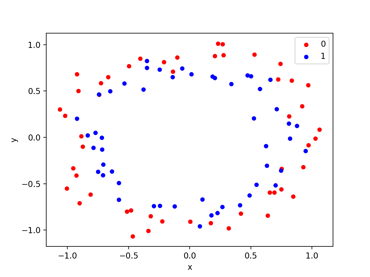
Scatter Plot of Circles Dataset with Color Showing the Class Value of Each Sample

This is a good test problem because the classes cannot be separated by a line, e.g. are not linearly separable, requiring a nonlinear method such as a neural network to address.

We have only generated 100 samples, which is small for a neural network, providing the opportunity to overfit the training dataset and have higher error on the test dataset: a good case for using regularization. Further, the samples have noise, giving the model an opportunity to learn aspects of the samples that don’t generalize.

Overfit Multilayer Perceptron

We can develop an MLP model to address this binary classification problem.

The model will have one hidden layer with more nodes than may be required to solve this problem, providing an opportunity to overfit. We will also train the model for longer than is required to ensure the model overfits.

Before we define the model, we will split the dataset into train and test sets, using 30 examples to train the model and 70 to evaluate the fit model’s performance.

# generate 2d classification dataset
X, y = make_circles(n_samples=100, noise=0.1, random_state=1)
# split into train and test
n_train = 30
trainX, testX = X[:n_train, :], X[n_train:, :]
trainy, testy = y[:n_train], y[n_train:]

Next, we can define the model.

The hidden layer uses 500 nodes in the hidden layer and the rectified linear activation function. A sigmoid activation function is used in the output layer in order to predict class values of 0 or 1.

The model is optimized using the binary cross entropy loss function, suitable for binary classification problems and the efficient Adam version of gradient descent.

# define model
model = Sequential()
model.add(Dense(500, input_dim=2, activation='relu'))
model.add(Dense(1, activation='sigmoid'))
model.compile(loss='binary_crossentropy', optimizer='adam', metrics=['accuracy'])

The defined model is then fit on the training data for 4,000 epochs and the default batch size of 32.

We will also use the test dataset as a validation dataset.

# fit model
history = model.fit(trainX, trainy, validation_data=(testX, testy), epochs=4000, verbose=0)

We can evaluate the performance of the model on the test dataset and report the result.

# evaluate the model
_, train_acc = model.evaluate(trainX, trainy, verbose=0)
_, test_acc = model.evaluate(testX, testy, verbose=0)
print('Train: %.3f, Test: %.3f' % (train_acc, test_acc))

Finally, we will plot the performance of the model on both the train and test set each epoch.

If the model does indeed overfit the training dataset, we would expect the line plot of accuracy on the training set to continue to increase and the test set to rise and then fall again as the model learns statistical noise in the training dataset.

# plot history
pyplot.plot(history.history['acc'], label='train')
pyplot.plot(history.history['val_acc'], label='test')
pyplot.legend()
pyplot.show()

We can tie all of these pieces together; the complete example is listed below.

# mlp overfit on the two circles dataset
from sklearn.datasets import make_circles
from keras.layers import Dense
from keras.models import Sequential
from matplotlib import pyplot
# generate 2d classification dataset
X, y = make_circles(n_samples=100, noise=0.1, random_state=1)
# split into train and test
n_train = 30
trainX, testX = X[:n_train, :], X[n_train:, :]
trainy, testy = y[:n_train], y[n_train:]
# define model
model = Sequential()
model.add(Dense(500, input_dim=2, activation='relu'))
model.add(Dense(1, activation='sigmoid'))
model.compile(loss='binary_crossentropy', optimizer='adam', metrics=['accuracy'])
# fit model
history = model.fit(trainX, trainy, validation_data=(testX, testy), epochs=4000, verbose=0)
# evaluate the model
_, train_acc = model.evaluate(trainX, trainy, verbose=0)
_, test_acc = model.evaluate(testX, testy, verbose=0)
print('Train: %.3f, Test: %.3f' % (train_acc, test_acc))
# plot history
pyplot.plot(history.history['acc'], label='train')
pyplot.plot(history.history['val_acc'], label='test')
pyplot.legend()
pyplot.show()

Running the example reports the model performance on the train and test datasets.

We can see that the model has better performance on the training dataset than the test dataset, one possible sign of overfitting.

Your specific results may vary given the stochastic nature of the neural network and the training algorithm. Because the model is severely overfit, we generally would not expect much, if any, variance in the accuracy across repeated runs of the model on the same dataset.

Train: 1.000, Test: 0.757

A figure is created showing line plots of the model accuracy on the train and test sets.

We can see that expected shape of an overfit model where test accuracy increases to a point and then begins to decrease again.

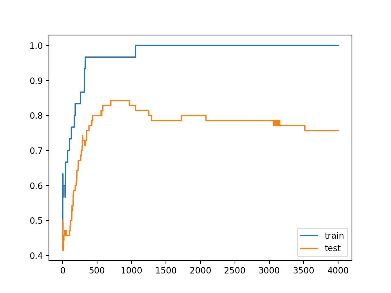
Line Plots of Accuracy on Train and Test Datasets While Training Showing an Overfit

Overfit MLP With Dropout Regularization

We can update the example to use dropout regularization.

We can do this by simply inserting a new Dropout layer between the hidden layer and the output layer. In this case, we will specify a dropout rate (probability of setting outputs from the hidden layer to zero) to 40% or 0.4.

# define model
model = Sequential()
model.add(Dense(500, input_dim=2, activation='relu'))
model.add(Dropout(0.4))
model.add(Dense(1, activation='sigmoid'))
model.compile(loss='binary_crossentropy', optimizer='adam', metrics=['accuracy'])

The complete updated example with the addition of dropout after the hidden layer is listed below:

# mlp with dropout on the two circles dataset
from sklearn.datasets import make_circles
from keras.models import Sequential
from keras.layers import Dense
from keras.layers import Dropout
from matplotlib import pyplot
# generate 2d classification dataset
X, y = make_circles(n_samples=100, noise=0.1, random_state=1)
# split into train and test
n_train = 30
trainX, testX = X[:n_train, :], X[n_train:, :]
trainy, testy = y[:n_train], y[n_train:]
# define model
model = Sequential()
model.add(Dense(500, input_dim=2, activation='relu'))
model.add(Dropout(0.4))
model.add(Dense(1, activation='sigmoid'))
model.compile(loss='binary_crossentropy', optimizer='adam', metrics=['accuracy'])
# fit model
history = model.fit(trainX, trainy, validation_data=(testX, testy), epochs=4000, verbose=0)
# evaluate the model
_, train_acc = model.evaluate(trainX, trainy, verbose=0)
_, test_acc = model.evaluate(testX, testy, verbose=0)
print('Train: %.3f, Test: %.3f' % (train_acc, test_acc))
# plot history
pyplot.plot(history.history['acc'], label='train')
pyplot.plot(history.history['val_acc'], label='test')
pyplot.legend()
pyplot.show()

Running the example reports the model performance on the train and test datasets.

Your results will likely vary. In this case, the resulting model has a high variance.

In this specific case, we can see that dropout resulted in a slight drop in accuracy on the training dataset, down from 100% to 96%, and a lift in accuracy on the test set, up from 75% to 81%.

Train: 0.967, Test: 0.814

Reviewing the line plot of train and test accuracy during training, we can see that it no longer appears that the model has overfit the training dataset.

Model accuracy on both the train and test sets continues to increase to a plateau, albeit with a lot of noise given the use of dropout during training.

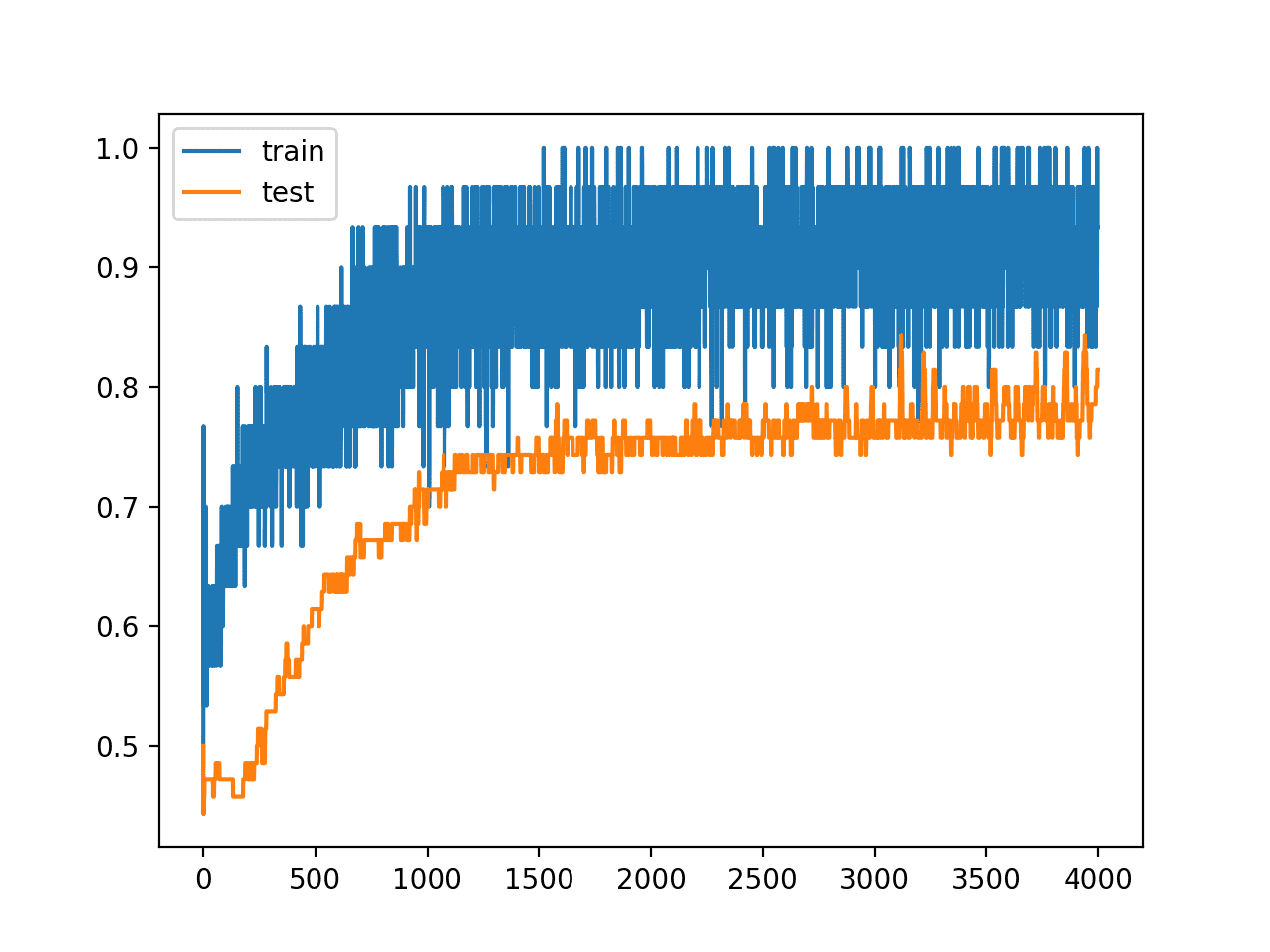
Line Plots of Accuracy on Train and Test Datasets While Training With Dropout Regularization

Extensions

This section lists some ideas for extending the tutorial that you may wish to explore.

Input Dropout. Update the example to use dropout on the input variables and compare results.
Weight Constraint. Update the example to add a max-norm weight constraint to the hidden layer and compare results.
Repeated Evaluation. Update the example to repeat the evaluation of the overfit and dropout model and summarize and compare the average results.
Grid Search Rate. Develop a grid search of dropout probabilities and report the relationship between dropout rate and test set accuracy.

If you explore any of these extensions, I’d love to know.

Summary

In this tutorial, you discovered the Keras API for adding dropout regularization to deep learning neural network models.

Specifically, you learned:

How to create a dropout layer using the Keras API.
How to add dropout regularization to MLP, CNN, and RNN layers using the Keras API.
How to reduce overfitting by adding a dropout regularization to an existing model.

Do you have any questions?
Ask your questions in the comments below and I will do my best to answer.

The post How to Reduce Overfitting With Dropout Regularization in Keras appeared first on Machine Learning Mastery.

Go to Source