
Author: Jason Brownlee
A problem with training neural networks is in the choice of the number of training epochs to use.
Too many epochs can lead to overfitting of the training dataset, whereas too few may result in an underfit model. Early stopping is a method that allows you to specify an arbitrary large number of training epochs and stop training once the model performance stops improving on a hold out validation dataset.
In this tutorial, you will discover the Keras API for adding early stopping to overfit deep learning neural network models.
After completing this tutorial, you will know:
- How to monitor the performance of a model during training using the Keras API.
- How to create and configure early stopping and model checkpoint callbacks using the Keras API.
- How to reduce overfitting by adding an early stopping to an existing model.
Let’s get started.

How to Stop Training Deep Neural Networks At the Right Time With Using Early Stopping
Photo by Ian D. Keating, some rights reserved.
Tutorial Overview
This tutorial is divided into six parts; they are:
- Using Callbacks in Keras
- Evaluating a Validation Dataset
- Monitoring Model Performance
- Early Stopping in Keras
- Checkpointing in Keras
- Early Stopping Case Study
Using Callbacks in Keras
Callbacks provide a way to execute code and interact with the training model process automatically.
Callbacks can be provided to the fit() function via the “callbacks” argument.
First, callbacks must be instantiated.
...
cb = Callback(...)
Then, one or more callbacks that you intend to use must be added to a Python list.
...
cb_list = [cb, ...]
Finally, the list of callbacks is provided to the callback argument when fitting the model.
...
model.fit(..., callbacks=cb_list)
Evaluating a Validation Dataset in Keras
Early stopping requires that a validation dataset is evaluated during training.
This can be achieved by specifying the validation dataset to the fit() function when training your model.
There are two ways of doing this.
The first involves you manually splitting your training data into a train and validation dataset and specifying the validation dataset to the fit() function via the validation_data argument. For example:
...
model.fit(train_X, train_y, validation_data=(val_x, val_y))
Alternately, the fit() function can automatically split your training dataset into train and validation sets based on a percentage split specified via the validation_split argument.
The validation_split is a value between 0 and 1 and defines the percentage amount of the training dataset to use for the validation dataset. For example:
...
model.fit(train_X, train_y, validation_split=0.3)
In both cases, the model is not trained on the validation dataset. Instead, the model is evaluated on the validation dataset at the end of each training epoch.
Monitoring Model Performance
The loss function chosen to be optimized for your model is calculated at the end of each epoch.
To callbacks, this is made available via the name “loss.”
If a validation dataset is specified to the fit() function via the validation_data or validation_split arguments, then the loss on the validation dataset will be made available via the name “val_loss.”
Additional metrics can be monitored during the training of the model.
They can be specified when compiling the model via the “metrics” argument to the compile function. This argument takes a Python list of known metric functions, such as ‘mse‘ for mean squared error and ‘acc‘ for accuracy. For example:
...
model.compile(..., metrics=['acc'])
If additional metrics are monitored during training, they are also available to the callbacks via the same name, such as ‘acc‘ for accuracy on the training dataset and ‘val_acc‘ for the accuracy on the validation dataset. Or, ‘mse‘ for mean squared error on the training dataset and ‘val_mse‘ on the validation dataset.
Early Stopping in Keras
Keras supports the early stopping of training via a callback called EarlyStopping.
This callback allows you to specify the performance measure to monitor, the trigger, and once triggered, it will stop the training process.
The EarlyStopping callback is configured when instantiated via arguments.
The “monitor” allows you to specify the performance measure to monitor in order to end training. Recall from the previous section that the calculation of measures on the validation dataset will have the ‘val_‘ prefix, such as ‘val_loss‘ for the loss on the validation dataset.
es = EarlyStopping(monitor='val_loss')
Based on the choice of performance measure, the “mode” argument will need to be specified as whether the objective of the chosen metric is to increase (maximize or ‘max‘) or to decrease (minimize or ‘min‘).
For example, we would seek a minimum for validation loss and a minimum for validation mean squared error, whereas we would seek a maximum for validation accuracy.
es = EarlyStopping(monitor='val_loss', mode='min')
By default, mode is set to ‘auto‘ and knows that you want to minimize loss or maximize accuracy.
That is all that is needed for the simplest form of early stopping. Training will stop when the chosen performance measure stops improving. To discover the training epoch on which training was stopped, the “verbose” argument can be set to 1. Once stopped, the callback will print the epoch number.
es = EarlyStopping(monitor='val_loss', mode='min', verbose=1)
Often, the first sign of no further improvement may not be the best time to stop training. This is because the model may coast into a plateau of no improvement or even get slightly worse before getting much better.
We can account for this by adding a delay to the trigger in terms of the number of epochs on which we would like to see no improvement. This can be done by setting the “patience” argument.
es = EarlyStopping(monitor='val_loss', mode='min', verbose=1, patience=50)
The exact amount of patience will vary between models and problems. Reviewing plots of your performance measure can be very useful to get an idea of how noisy the optimization process for your model on your data may be.
By default, any change in the performance measure, no matter how fractional, will be considered an improvement. You may want to consider an improvement that is a specific increment, such as 1 unit for mean squared error or 1% for accuracy. This can be specified via the “min_delta” argument.
es = EarlyStopping(monitor='val_acc', mode='max', min_delta=1)
Finally, it may be desirable to only stop training if performance stays above or below a given threshold or baseline. For example, if you have familiarity with the training of the model (e.g. learning curves) and know that once a validation loss of a given value is achieved that there is no point in continuing training. This can be specified by setting the “baseline” argument.
This might be more useful when fine tuning a model, after the initial wild fluctuations in the performance measure seen in the early stages of training a new model are past.
es = EarlyStopping(monitor='val_loss', mode='min', baseline=0.4)
Checkpointing in Keras
The EarlyStopping callback will stop training once triggered, but the model at the end of training may not be the model with best performance on the validation dataset.
An additional callback is required that will save the best model observed during training for later use. This is the ModelCheckpoint callback.
The ModelCheckpoint callback is flexible in the way it can be used, but in this case we will use it only to save the best model observed during training as defined by a chosen performance measure on the validation dataset.
Saving and loading models requires that HDF5 support has been installed on your workstation. For example, using the pip Python installer, this can be achieved as follows:
sudo pip install h5py
You can learn more from the h5py Installation documentation.
The callback will save the model to file, which requires that a path and filename be specified via the first argument.
mc = ModelCheckpoint('best_model.h5')
The preferred loss function to be monitored can be specified via the monitor argument, in the same way as the EarlyStopping callback. For example, loss on the validation dataset (the default).
mc = ModelCheckpoint('best_model.h5', monitor='val_loss')
Also, as with the EarlyStopping callback, we must specify the “mode” as either minimizing or maximizing the performance measure. Again, the default is ‘auto,’ which is aware of the standard performance measures.
mc = ModelCheckpoint('best_model.h5', monitor='val_loss', mode='min')
Finally, we are interested in only the very best model observed during training, rather than the best compared to the previous epoch, which might not be the best overall if training is noisy. This can be achieved by setting the “save_best_only” argument to True.
mc = ModelCheckpoint('best_model.h5', monitor='val_loss', mode='min', save_best_only=True)
That is all that is needed to ensure the model with the best performance is saved when using early stopping, or in general.
It may be interesting to know the value of the performance measure and at what epoch the model was saved. This can be printed by the callback by setting the “verbose” argument to “1“.
mc = ModelCheckpoint('best_model.h5', monitor='val_loss', mode='min', verbose=1)
The saved model can then be loaded and evaluated any time by calling the load_model() function.
# load a saved model
from keras.models import load_model
saved_model = load_model('best_model.h5')
Now that we know how to use the early stopping and model checkpoint APIs, let’s look at a worked example.
Early Stopping Case Study
In this section, we will demonstrate how to use early stopping to reduce overfitting of an MLP on a simple binary classification problem.
This example provides a template for applying early stopping to your own neural network for classification and regression problems.
Binary Classification Problem
We will use a standard binary classification problem that defines two semi-circles of observations, one semi-circle for each class.
Each observation has two input variables with the same scale and a class output value of either 0 or 1. This dataset is called the “moons” dataset because of the shape of the observations in each class when plotted.
We can use the make_moons() function to generate observations from this problem. We will add noise to the data and seed the random number generator so that the same samples are generated each time the code is run.
# generate 2d classification dataset
X, y = make_moons(n_samples=100, noise=0.2, random_state=1)
We can plot the dataset where the two variables are taken as x and y coordinates on a graph and the class value is taken as the color of the observation.
The complete example of generating the dataset and plotting it is listed below.
# generate two moons dataset
from sklearn.datasets import make_moons
from matplotlib import pyplot
from pandas import DataFrame
# generate 2d classification dataset
X, y = make_moons(n_samples=100, noise=0.2, random_state=1)
# scatter plot, dots colored by class value
df = DataFrame(dict(x=X[:,0], y=X[:,1], label=y))
colors = {0:'red', 1:'blue'}
fig, ax = pyplot.subplots()
grouped = df.groupby('label')
for key, group in grouped:
    group.plot(ax=ax, kind='scatter', x='x', y='y', label=key, color=colors[key])
pyplot.show()
Running the example creates a scatter plot showing the semi-circle or moon shape of the observations in each class. We can see the noise in the dispersal of the points making the moons less obvious.
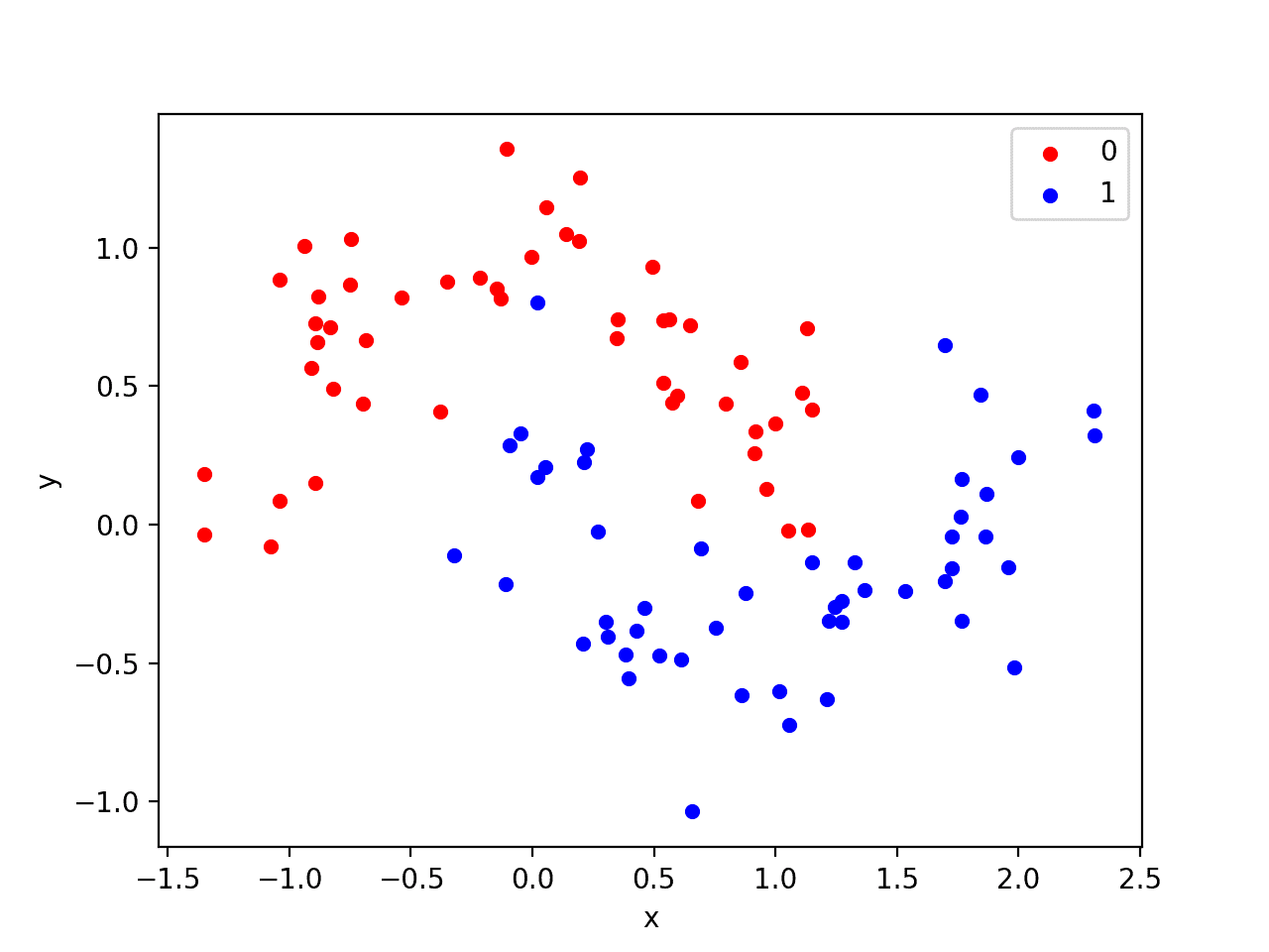
Scatter Plot of Moons Dataset With Color Showing the Class Value of Each Sample
This is a good test problem because the classes cannot be separated by a line, e.g. are not linearly separable, requiring a nonlinear method such as a neural network to address.
We have only generated 100 samples, which is small for a neural network, providing the opportunity to overfit the training dataset and have higher error on the test dataset: a good case for using regularization. Further, the samples have noise, giving the model an opportunity to learn aspects of the samples that don’t generalize.
Overfit Multilayer Perceptron
We can develop an MLP model to address this binary classification problem.
The model will have one hidden layer with more nodes than may be required to solve this problem, providing an opportunity to overfit. We will also train the model for longer than is required to ensure the model overfits.
Before we define the model, we will split the dataset into train and test sets, using 30 examples to train the model and 70 to evaluate the fit model’s performance.
# generate 2d classification dataset
X, y = make_moons(n_samples=100, noise=0.2, random_state=1)
# split into train and test
n_train = 30
trainX, testX = X[:n_train, :], X[n_train:, :]
trainy, testy = y[:n_train], y[n_train:]
Next, we can define the model.
The hidden layer uses 500 nodes and the rectified linear activation function. A sigmoid activation function is used in the output layer in order to predict class values of 0 or 1. The model is optimized using the binary cross entropy loss function, suitable for binary classification problems and the efficient Adam version of gradient descent.
# define model
model = Sequential()
model.add(Dense(500, input_dim=2, activation='relu'))
model.add(Dense(1, activation='sigmoid'))
model.compile(loss='binary_crossentropy', optimizer='adam', metrics=['accuracy'])
The defined model is then fit on the training data for 4,000 epochs and the default batch size of 32.
We will also use the test dataset as a validation dataset. This is just a simplification for this example. In practice, you would split the training set into train and validation and also hold back a test set for final model evaluation.
# fit model
history = model.fit(trainX, trainy, validation_data=(testX, testy), epochs=4000, verbose=0)
We can evaluate the performance of the model on the test dataset and report the result.
# evaluate the model
_, train_acc = model.evaluate(trainX, trainy, verbose=0)
_, test_acc = model.evaluate(testX, testy, verbose=0)
print('Train: %.3f, Test: %.3f' % (train_acc, test_acc))
Finally, we will plot the loss of the model on both the train and test set each epoch.
If the model does indeed overfit the training dataset, we would expect the line plot of loss (and accuracy) on the training set to continue to increase and the test set to rise and then fall again as the model learns statistical noise in the training dataset.
# plot training history
pyplot.plot(history.history['loss'], label='train')
pyplot.plot(history.history['val_loss'], label='test')
pyplot.legend()
pyplot.show()
We can tie all of these pieces together; the complete example is listed below.
# mlp overfit on the moons dataset
from sklearn.datasets import make_moons
from keras.layers import Dense
from keras.models import Sequential
from matplotlib import pyplot
# generate 2d classification dataset
X, y = make_moons(n_samples=100, noise=0.2, random_state=1)
# split into train and test
n_train = 30
trainX, testX = X[:n_train, :], X[n_train:, :]
trainy, testy = y[:n_train], y[n_train:]
# define model
model = Sequential()
model.add(Dense(500, input_dim=2, activation='relu'))
model.add(Dense(1, activation='sigmoid'))
model.compile(loss='binary_crossentropy', optimizer='adam', metrics=['accuracy'])
# fit model
history = model.fit(trainX, trainy, validation_data=(testX, testy), epochs=4000, verbose=0)
# evaluate the model
_, train_acc = model.evaluate(trainX, trainy, verbose=0)
_, test_acc = model.evaluate(testX, testy, verbose=0)
print('Train: %.3f, Test: %.3f' % (train_acc, test_acc))
# plot training history
pyplot.plot(history.history['loss'], label='train')
pyplot.plot(history.history['val_loss'], label='test')
pyplot.legend()
pyplot.show()
Running the example reports the model performance on the train and test datasets.
We can see that the model has better performance on the training dataset than the test dataset, one possible sign of overfitting.
Your specific results may vary given the stochastic nature of the neural network and the training algorithm. Because the model is severely overfit, we generally would not expect much, if any, variance in the accuracy across repeated runs of the model on the same dataset.
Train: 1.000, Test: 0.914
A figure is created showing line plots of the model loss on the train and test sets.
We can see that expected shape of an overfit model where test accuracy increases to a point and then begins to decrease again.
Reviewing the figure, we can also see flat spots in the ups and downs in the validation loss. Any early stopping will have to account for these behaviors. We would also expect that a good time to stop training might be around epoch 800.
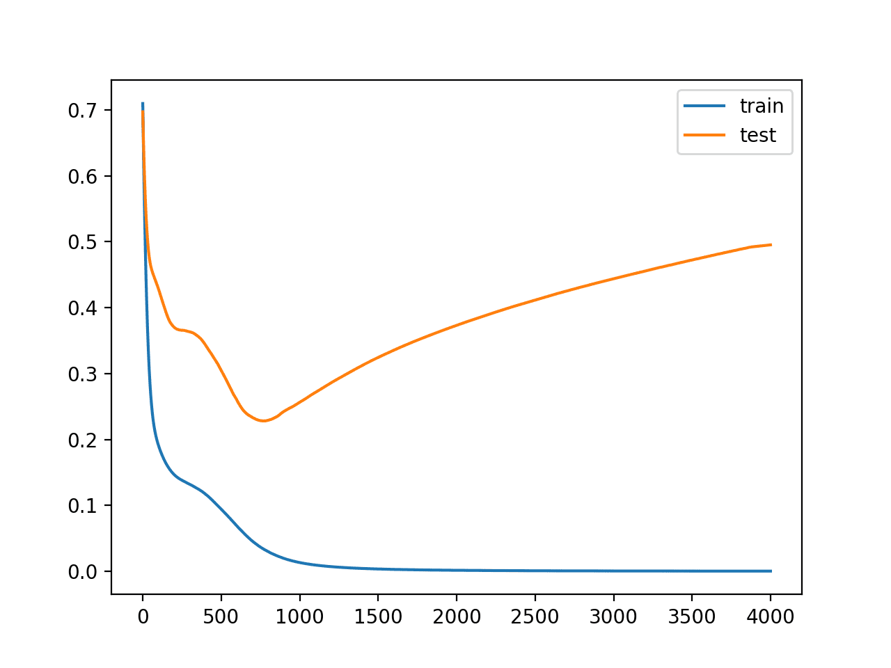
Line Plots of Loss on Train and Test Datasets While Training Showing an Overfit Model
Overfit MLP With Early Stopping
We can update the example and add very simple early stopping.
As soon as the loss of the model begins to increase on the test dataset, we will stop training.
First, we can define the early stopping callback.
# simple early stopping
es = EarlyStopping(monitor='val_loss', mode='min', verbose=1)
We can then update the call to the fit() function and specify a list of callbacks via the “callback” argument.
# fit model
history = model.fit(trainX, trainy, validation_data=(testX, testy), epochs=4000, verbose=0, callbacks=[es])
The complete example with the addition of simple early stopping is listed below.
# mlp overfit on the moons dataset with simple early stopping
from sklearn.datasets import make_moons
from keras.models import Sequential
from keras.layers import Dense
from keras.callbacks import EarlyStopping
from matplotlib import pyplot
# generate 2d classification dataset
X, y = make_moons(n_samples=100, noise=0.2, random_state=1)
# split into train and test
n_train = 30
trainX, testX = X[:n_train, :], X[n_train:, :]
trainy, testy = y[:n_train], y[n_train:]
# define model
model = Sequential()
model.add(Dense(500, input_dim=2, activation='relu'))
model.add(Dense(1, activation='sigmoid'))
model.compile(loss='binary_crossentropy', optimizer='adam', metrics=['accuracy'])
# simple early stopping
es = EarlyStopping(monitor='val_loss', mode='min', verbose=1)
# fit model
history = model.fit(trainX, trainy, validation_data=(testX, testy), epochs=4000, verbose=0, callbacks=[es])
# evaluate the model
_, train_acc = model.evaluate(trainX, trainy, verbose=0)
_, test_acc = model.evaluate(testX, testy, verbose=0)
print('Train: %.3f, Test: %.3f' % (train_acc, test_acc))
# plot training history
pyplot.plot(history.history['loss'], label='train')
pyplot.plot(history.history['val_loss'], label='test')
pyplot.legend()
pyplot.show()
Running the example reports the model performance on the train and test datasets.
We can also see that the callback stopped training at epoch 200. This is too early as we would expect an early stop to be around epoch 800. This is also highlighted by the classification accuracy on both the train and test sets, which is worse than no early stopping.
Epoch 00219: early stopping
Train: 0.967, Test: 0.814
Reviewing the line plot of train and test loss, we can indeed see that training was stopped at the point when validation loss began to plateau for the first time.
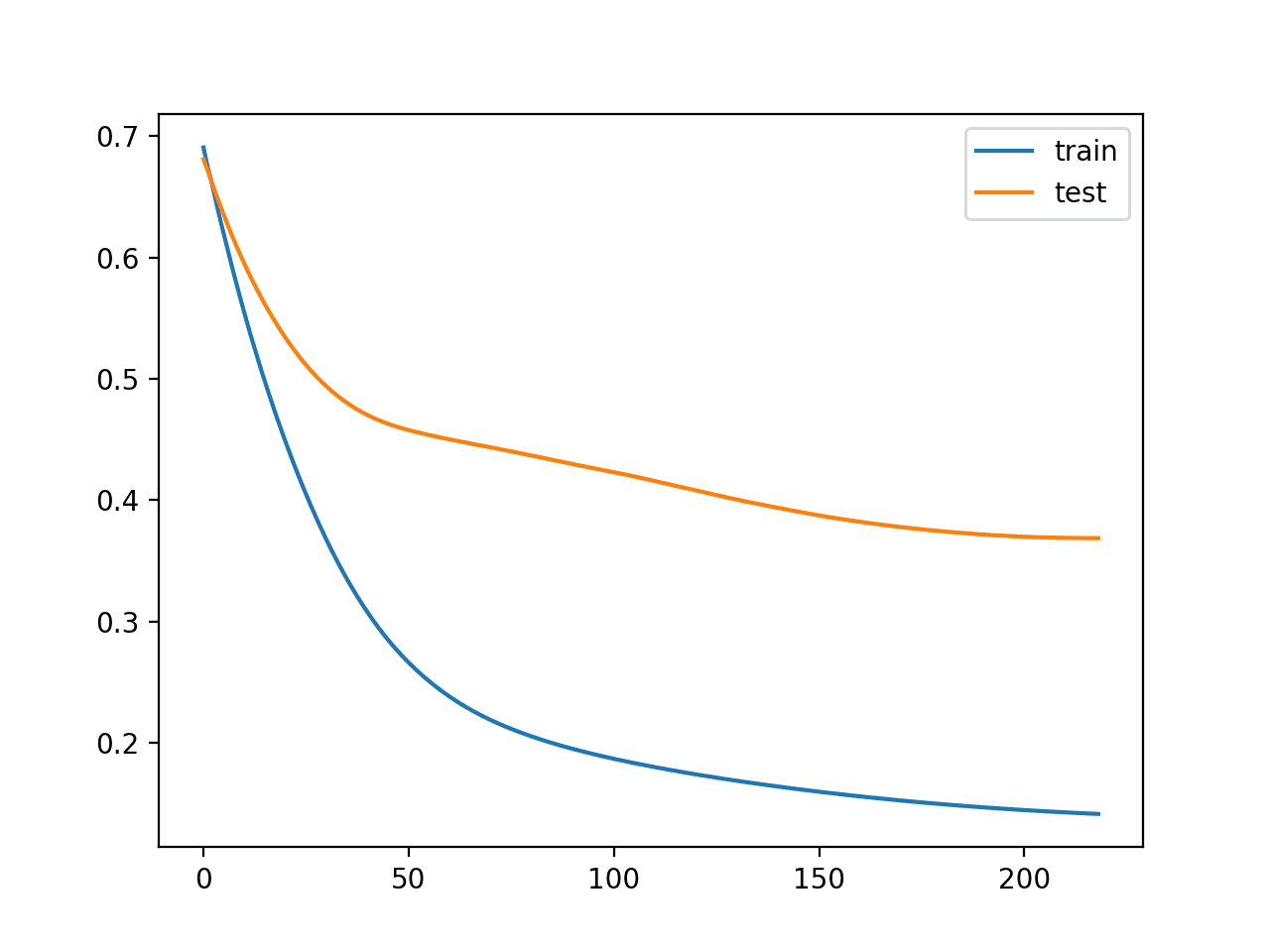
Line Plot of Train and Test Loss During Training With Simple Early Stopping
We can improve the trigger for early stopping by waiting a while before stopping.
This can be achieved by setting the “patience” argument.
In this case, we will wait 200 epochs before training is stopped. Specifically, this means that we will allow training to continue for up to an additional 200 epochs after the point that validation loss started to degrade, giving the training process an opportunity to get across flat spots or find some additional improvement.
# patient early stopping
es = EarlyStopping(monitor='val_loss', mode='min', verbose=1, patience=200)
The complete example with this change is listed below.
# mlp overfit on the moons dataset with patient early stopping
from sklearn.datasets import make_moons
from keras.models import Sequential
from keras.layers import Dense
from keras.callbacks import EarlyStopping
from matplotlib import pyplot
# generate 2d classification dataset
X, y = make_moons(n_samples=100, noise=0.2, random_state=1)
# split into train and test
n_train = 30
trainX, testX = X[:n_train, :], X[n_train:, :]
trainy, testy = y[:n_train], y[n_train:]
# define model
model = Sequential()
model.add(Dense(500, input_dim=2, activation='relu'))
model.add(Dense(1, activation='sigmoid'))
model.compile(loss='binary_crossentropy', optimizer='adam', metrics=['accuracy'])
# patient early stopping
es = EarlyStopping(monitor='val_loss', mode='min', verbose=1, patience=200)
# fit model
history = model.fit(trainX, trainy, validation_data=(testX, testy), epochs=4000, verbose=0, callbacks=[es])
# evaluate the model
_, train_acc = model.evaluate(trainX, trainy, verbose=0)
_, test_acc = model.evaluate(testX, testy, verbose=0)
print('Train: %.3f, Test: %.3f' % (train_acc, test_acc))
# plot training history
pyplot.plot(history.history['loss'], label='train')
pyplot.plot(history.history['val_loss'], label='test')
pyplot.legend()
pyplot.show()
Running the example, we can see that training was stopped much later, in this case after epoch 1,000. Your specific results may differ given the stochastic nature of training neural networks.
We can also see that the performance on the test dataset is better than not using any early stopping.
Epoch 01033: early stopping
Train: 1.000, Test: 0.943
Reviewing the line plot of loss during training, we can see that the patience allowed the training to progress past some small flat and bad spots.
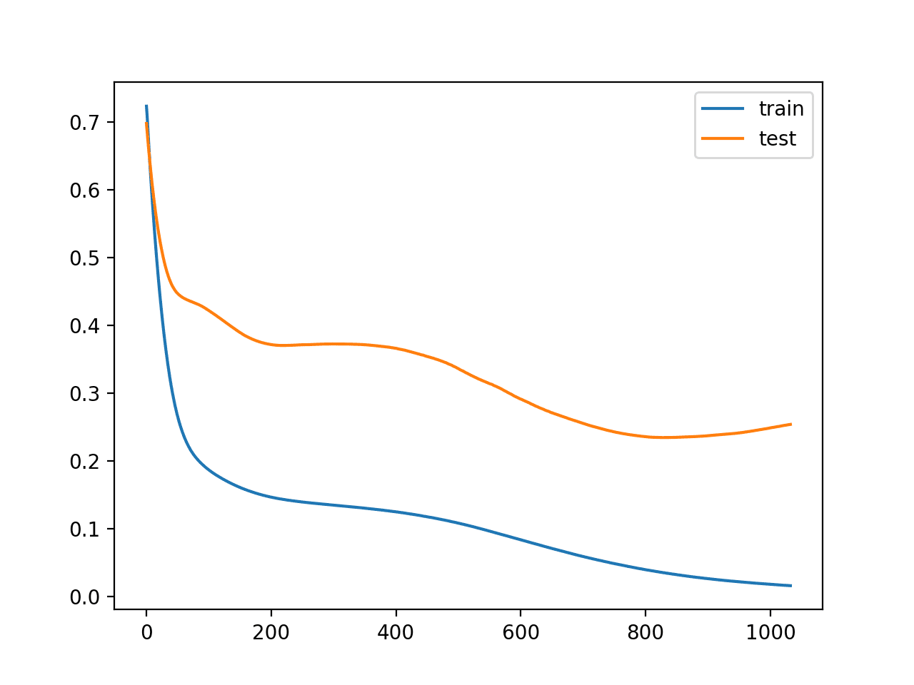
Line Plot of Train and Test Loss During Training With Patient Early Stopping
We can also see that test loss started to increase again in the last approximately 100 epochs.
This means that although the performance of the model has improved, we may not have the best performing or most stable model at the end of training. We can address this by using a ModelChecckpoint callback.
In this case, we are interested in saving the model with the best accuracy on the test dataset. We could also seek the model with the best loss on the test dataset, but this may or may not correspond to the model with the best accuracy.
This highlights an important concept in model selection. The notion of the “best” model during training may conflict when evaluated using different performance measures. Try to choose models based on the metric by which they will be evaluated and presented in the domain. In a balanced binary classification problem, this will most likely be classification accuracy. Therefore, we will use accuracy on the validation in the ModelCheckpoint callback to save the best model observed during training.
mc = ModelCheckpoint('best_model.h5', monitor='val_acc', mode='max', verbose=1, save_best_only=True)
During training, the entire model will be saved to the file “best_model.h5” only when accuracy on the validation dataset improves overall across the entire training process. A verbose output will also inform us as to the epoch and accuracy value each time the model is saved to the same file (e.g. overwritten).
This new additional callback can be added to the list of callbacks when calling the fit() function.
history = model.fit(trainX, trainy, validation_data=(testX, testy), epochs=4000, verbose=0, callbacks=[es, mc])
We are no longer interested in the line plot of loss during training; it will be much the same as the previous run.
Instead, we want to load the saved model from file and evaluate its performance on the test dataset.
# load the saved model
saved_model = load_model('best_model.h5')
# evaluate the model
_, train_acc = saved_model.evaluate(trainX, trainy, verbose=0)
_, test_acc = saved_model.evaluate(testX, testy, verbose=0)
print('Train: %.3f, Test: %.3f' % (train_acc, test_acc))
The complete example with these changes is listed below.
# mlp overfit on the moons dataset with patient early stopping and model checkpointing
from sklearn.datasets import make_moons
from keras.models import Sequential
from keras.layers import Dense
from keras.callbacks import EarlyStopping
from keras.callbacks import ModelCheckpoint
from matplotlib import pyplot
from keras.models import load_model
# generate 2d classification dataset
X, y = make_moons(n_samples=100, noise=0.2, random_state=1)
# split into train and test
n_train = 30
trainX, testX = X[:n_train, :], X[n_train:, :]
trainy, testy = y[:n_train], y[n_train:]
# define model
model = Sequential()
model.add(Dense(500, input_dim=2, activation='relu'))
model.add(Dense(1, activation='sigmoid'))
model.compile(loss='binary_crossentropy', optimizer='adam', metrics=['accuracy'])
# simple early stopping
es = EarlyStopping(monitor='val_loss', mode='min', verbose=1, patience=200)
mc = ModelCheckpoint('best_model.h5', monitor='val_acc', mode='max', verbose=1, save_best_only=True)
# fit model
history = model.fit(trainX, trainy, validation_data=(testX, testy), epochs=4000, verbose=0, callbacks=[es, mc])
# load the saved model
saved_model = load_model('best_model.h5')
# evaluate the model
_, train_acc = saved_model.evaluate(trainX, trainy, verbose=0)
_, test_acc = saved_model.evaluate(testX, testy, verbose=0)
print('Train: %.3f, Test: %.3f' % (train_acc, test_acc))
Running the example, we can see the verbose output from the ModelCheckpoint callback for both when a new best model is saved and from when no improvement was observed.
We can see that the best model was observed at epoch 879 during this run. Your specific results may vary given the stochastic nature of training neural networks.
Again, we can see that early stopping continued patiently until after epoch 1,000. Note that epoch 880 + a patience of 200 is not epoch 1044. Recall that early stopping is monitoring loss on the validation dataset and that the model checkpoint is saving models based on accuracy. As such, the patience of early stopping started at an epoch other than 880.
...
Epoch 00878: val_acc did not improve from 0.92857
Epoch 00879: val_acc improved from 0.92857 to 0.94286, saving model to best_model.h5
Epoch 00880: val_acc did not improve from 0.94286
...
Epoch 01042: val_acc did not improve from 0.94286
Epoch 01043: val_acc did not improve from 0.94286
Epoch 01044: val_acc did not improve from 0.94286
Epoch 01044: early stopping
Train: 1.000, Test: 0.943
In this case, we don’t see any further improvement in model accuracy on the test dataset. Nevertheless, we have followed a good practice.
Why not monitor validation accuracy for early stopping?
This is a good question. The main reason is that accuracy is a coarse measure of model performance during training and that loss provides more nuance when using early stopping with classification problems. The same measure may be used for early stopping and model checkpointing in the case of regression, such as mean squared error.
Extensions
This section lists some ideas for extending the tutorial that you may wish to explore.
- Use Accuracy. Update the example to monitor accuracy on the test dataset rather than loss, and plot learning curves showing accuracy.
- Use True Validation Set. Update the example to split the training set into train and validation sets, then evaluate the model on the test dataset.
- Regression Example. Create a new example of using early stopping to address overfitting on a simple regression problem and monitoring mean squared error.
If you explore any of these extensions, I’d love to know.
Further Reading
This section provides more resources on the topic if you are looking to go deeper.
Posts
- Avoid Overfitting by Early Stopping With XGBoost in Python
- How to Check-Point Deep Learning Models in Keras
API
- H5Py Installation Documentation
- Keras Regularizers API
- Keras Core Layers API
- Keras Convolutional Layers API
- Keras Recurrent Layers API
- Keras Callbacks API
- sklearn.datasets.make_moons API
Summary
In this tutorial, you discovered the Keras API for adding early stopping to overfit deep learning neural network models.
Specifically, you learned:
- How to monitor the performance of a model during training using the Keras API.
- How to create and configure early stopping and model checkpoint callbacks using the Keras API.
- How to reduce overfitting by adding a early stopping to an existing model.
Do you have any questions?
Ask your questions in the comments below and I will do my best to answer.
The post How to Stop Training Deep Neural Networks At the Right Time Using Early Stopping appeared first on Machine Learning Mastery.