
Author: Jason Brownlee
Adding noise to an underconstrained neural network model with a small training dataset can have a regularizing effect and reduce overfitting.
Keras supports the addition of Gaussian noise via a separate layer called the GaussianNoise layer. This layer can be used to add noise to an existing model.
In this tutorial, you will discover how to add noise to deep learning models in Keras in order to reduce overfitting and improve model generalization.
After completing this tutorial, you will know:
- Noise can be added to a neural network model via the GaussianNoise layer.
- The GaussianNoise can be used to add noise to input values or between hidden layers.
- How to add a GaussianNoise layer in order to reduce overfitting in a Multilayer Perceptron model for classification.
Let’s get started.

How to Improve Deep Learning Model Robustness by Adding Noise
Photo by Michael Mueller, some rights reserved.
Tutorial Overview
This tutorial is divided into three parts; they are:
- Noise Regularization in Keras
- Noise Regularization in Models
- Noise Regularization Case Study
Noise Regularization in Keras
Keras supports the addition of noise to models via the GaussianNoise layer.
This is a layer that will add noise to inputs of a given shape. The noise has a mean of zero and requires that a standard deviation of the noise be specified as a parameter. For example:
# import noise layer
from keras.layers import GaussianNoise
# define noise layer
layer = GaussianNoise(0.1)
The output of the layer will have the same shape as the input, with the only modification being the addition of noise to the values.
Noise Regularization in Models
The GaussianNoise can be used in a few different ways with a neural network model.
Firstly, it can be used as an input layer to add noise to input variables directly. This is the traditional use of noise as a regularization method in neural networks.
Below is an example of defining a GaussianNoise layer as an input layer for a model that takes 2 input variables.
...
model.add(GaussianNoise(0.01, input_shape=(2,)))
...
Noise can also be added between hidden layers in the model. Given the flexibility of Keras, the noise can be added before or after the use of the activation function. It may make more sense to add it before the activation; nevertheless, both options are possible.
Below is an example of a GaussianNoise layer that adds noise to the linear output of a Dense layer before a rectified linear activation function, perhaps a more appropriate use of noise between hidden layers.
...
model.add(Dense(32))
model.add(GaussianNoise(0.1))
model.add(Activation('relu'))
model.add(Dense(32))
...
Noise can also be added after the activation function, much like using a noisy activation function. One downside of this usage is that the resulting values may be out-of-range from what the activation function may normally provide. For example, a value with added noise may be less than zero, whereas the relu activation function will only ever output values 0 or larger.
...
model.add(Dense(32, activation='reu'))
model.add(GaussianNoise(0.1))
model.add(Dense(32))
...
Let’s take a look at how noise regularization can be used with some common network types.
MLP Noise Regularization
The example below adds noise between two Dense fully connected layers.
# example of noise between fully connected layers
from keras.layers import Dense
from keras.layers import GaussianNoise
from keras.layers import Activation
...
model.add(Dense(32))
model.add(GaussianNoise(0.1))
model.add(Activation('relu'))
model.add(Dense(1))
...
CNN Noise Regularization
The example below adds noise after a pooling layer in a convolutional network.
# example of noise for a CNN
from keras.layers import Dense
from keras.layers import Conv2D
from keras.layers import MaxPooling2D
from keras.layers import GaussianNoise
...
model.add(Conv2D(32, (3,3)))
model.add(Conv2D(32, (3,3)))
model.add(MaxPooling2D())
model.add(GaussianNoise(0.1))
model.add(Dense(1))
...
RNN Dropout Regularization
The example below adds noise between an LSTM recurrent layer and a Dense fully connected layer.
# example of noise between LSTM and fully connected layers
from keras.layers import Dense
from keras.layers import Activation
from keras.layers import LSTM
from keras.layers import GaussianNoise
...
model.add(LSTM(32))
model.add(GaussianNoise(0.5))
model.add(Activation('relu'))
model.add(Dense(1))
...
Now that we have seen how to add noise to neural network models, let’s look at a case study of adding noise to an overfit model to reduce generalization error.
Want Better Results with Deep Learning?
Take my free 7-day email crash course now (with sample code).
Click to sign-up and also get a free PDF Ebook version of the course.
Noise Regularization Case Study
In this section, we will demonstrate how to use noise regularization to reduce overfitting of an MLP on a simple binary classification problem.
This example provides a template for applying noise regularization to your own neural network for classification and regression problems.
Binary Classification Problem
We will use a standard binary classification problem that defines two two-dimensional concentric circles of observations, one semi-circle for each class.
Each observation has two input variables with the same scale and a class output value of either 0 or 1. This dataset is called the “circles” dataset because of the shape of the observations in each class when plotted.
We can use the make_circles() function to generate observations from this problem. We will add noise to the data and seed the random number generator so that the same samples are generated each time the code is run.
# generate 2d classification dataset
X, y = make_circles(n_samples=100, noise=0.1, random_state=1)
We can plot the dataset where the two variables are taken as x and y coordinates on a graph and the class value is taken as the color of the observation.
The complete example of generating the dataset and plotting it is listed below.
# generate two circles dataset
from sklearn.datasets import make_circles
from matplotlib import pyplot
from pandas import DataFrame
# generate 2d classification dataset
X, y = make_circles(n_samples=100, noise=0.1, random_state=1)
# scatter plot, dots colored by class value
df = DataFrame(dict(x=X[:,0], y=X[:,1], label=y))
colors = {0:'red', 1:'blue'}
fig, ax = pyplot.subplots()
grouped = df.groupby('label')
for key, group in grouped:
    group.plot(ax=ax, kind='scatter', x='x', y='y', label=key, color=colors[key])
pyplot.show()
Running the example creates a scatter plot showing the concentric circles shape of the observations in each class. We can see the noise in the dispersal of the points making the circles less obvious.
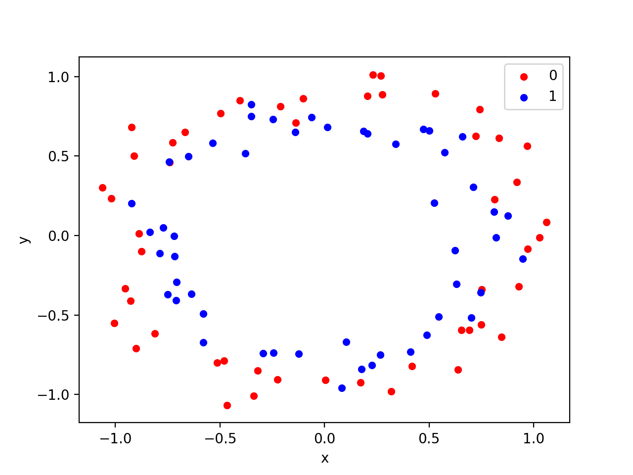
Scatter Plot of Circles Dataset with Color Showing the Class Value of Each Sample
This is a good test problem because the classes cannot be separated by a line, e.g. are not linearly separable, requiring a nonlinear method such as a neural network to address.
We have only generated 100 samples, which is small for a neural network, providing the opportunity to overfit the training dataset and have higher error on the test dataset, a good case for using regularization. Further, the samples have noise, giving the model an opportunity to learn aspects of the samples that don’t generalize.
Overfit Multilayer Perceptron
We can develop an MLP model to address this binary classification problem.
The model will have one hidden layer with more nodes than may be required to solve this problem, providing an opportunity to overfit. We will also train the model for longer than is required to ensure the model overfits.
Before we define the model, we will split the dataset into train and test sets, using 30 examples to train the model and 70 to evaluate the fit model’s performance.
# generate 2d classification dataset
X, y = make_circles(n_samples=100, noise=0.1, random_state=1)
# split into train and test
n_train = 30
trainX, testX = X[:n_train, :], X[n_train:, :]
trainy, testy = y[:n_train], y[n_train:]
Next, we can define the model.
The hidden layer uses 500 nodes in the hidden layer and the rectified linear activation function. A sigmoid activation function is used in the output layer in order to predict class values of 0 or 1. The model is optimized using the binary cross entropy loss function, suitable for binary classification problems and the efficient Adam version of gradient descent.
# define model
model = Sequential()
model.add(Dense(500, input_dim=2, activation='relu'))
model.add(Dense(1, activation='sigmoid'))
model.compile(loss='binary_crossentropy', optimizer='adam', metrics=['accuracy'])
The defined model is then fit on the training data for 4,000 epochs and the default batch size of 32.
We will also use the test dataset as a validation dataset.
# fit model
history = model.fit(trainX, trainy, validation_data=(testX, testy), epochs=4000, verbose=0)
We can evaluate the performance of the model on the test dataset and report the result.
# evaluate the model
_, train_acc = model.evaluate(trainX, trainy, verbose=0)
_, test_acc = model.evaluate(testX, testy, verbose=0)
print('Train: %.3f, Test: %.3f' % (train_acc, test_acc))
Finally, we will plot the performance of the model on both the train and test set each epoch.
If the model does indeed overfit the training dataset, we would expect the line plot of accuracy on the training set to continue to increase and the test set to rise and then fall again as the model learns statistical noise in the training dataset.
# plot history
pyplot.plot(history.history['acc'], label='train')
pyplot.plot(history.history['val_acc'], label='test')
pyplot.legend()
pyplot.show()
We can tie all of these pieces together; the complete example is listed below.
# mlp overfit on the two circles dataset
from sklearn.datasets import make_circles
from keras.layers import Dense
from keras.models import Sequential
from matplotlib import pyplot
# generate 2d classification dataset
X, y = make_circles(n_samples=100, noise=0.1, random_state=1)
# split into train and test
n_train = 30
trainX, testX = X[: n_train, :], X[n_train:, :]
trainy, testy = y[:n_train], y[n_train:]
# define model
model = Sequential()
model.add(Dense(500, input_dim=2, activation='relu'))
model.add(Dense(1, activation='sigmoid'))
model.compile(loss='binary_crossentropy', optimizer='adam', metrics=['accuracy'])
# fit model
history = model.fit(trainX, trainy, validation_data=(testX, testy), epochs=4000, verbose=0)
# evaluate the model
_, train_acc = model.evaluate(trainX, trainy, verbose=0)
_, test_acc = model.evaluate(testX, testy, verbose=0)
print('Train: %.3f, Test: %.3f' % (train_acc, test_acc))
# plot history
pyplot.plot(history.history['acc'], label='train')
pyplot.plot(history.history['val_acc'], label='test')
pyplot.legend()
pyplot.show()
Running the example reports the model performance on the train and test datasets.
We can see that the model has better performance on the training dataset than the test dataset, one possible sign of overfitting.
Your specific results may vary given the stochastic nature of the neural network and the training algorithm. Because the model is severely overfit, we generally would not expect much, if any, variance in the accuracy across repeated runs of the model on the same dataset.
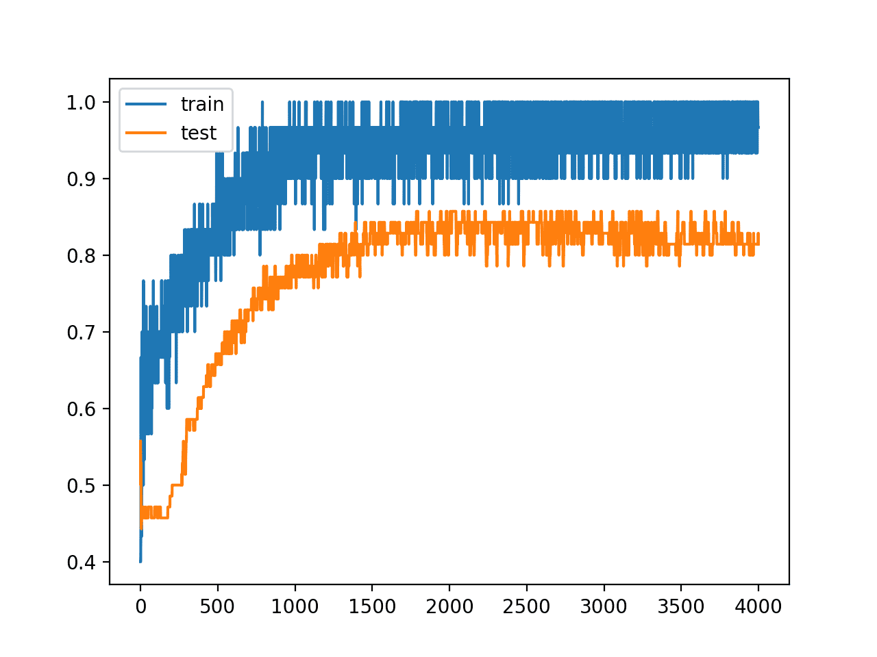
Train: 1.000, Test: 0.757
A figure is created showing line plots of the model accuracy on the train and test sets.
We can see that expected shape of an overfit model where test accuracy increases to a point and then begins to decrease again.
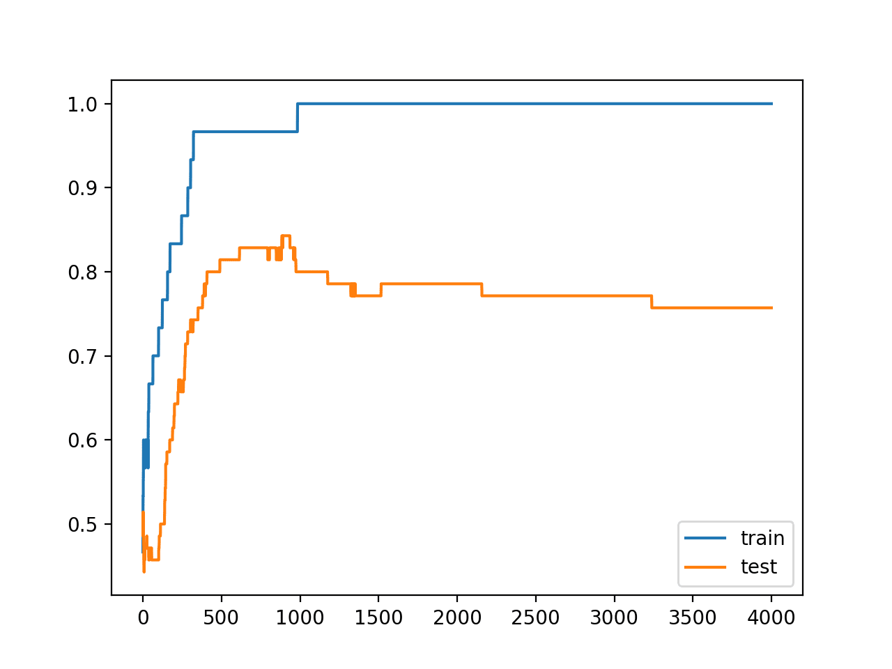
Line Plots of Accuracy on Train and Test Datasets While Training Showing an Overfit
MLP With Input Layer Noise
The dataset is defined by points that have a controlled amount of statistical noise.
Nevertheless, because the dataset is small, we can add further noise to the input values. This will have the effect of creating more samples or resampling the domain, making the structure of the input space artificially smoother. This may make the problem easier to learn and improve generalization performance.
We can add a GaussianNoise layer as the input layer. The amount of noise must be small. Given that the input values are within the range [0, 1], we will add Gaussian noise with a mean of 0.0 and a standard deviation of 0.01, chosen arbitrarily.
# define model
model = Sequential()
model.add(GaussianNoise(0.01, input_shape=(2,)))
model.add(Dense(500, activation='relu'))
model.add(Dense(1, activation='sigmoid'))
model.compile(loss='binary_crossentropy', optimizer='adam', metrics=['accuracy'])
The complete example with this change is listed below.
# mlp overfit on the two circles dataset with input noise
from sklearn.datasets import make_circles
from keras.models import Sequential
from keras.layers import Dense
from keras.layers import GaussianNoise
from matplotlib import pyplot
# generate 2d classification dataset
X, y = make_circles(n_samples=100, noise=0.1, random_state=1)
# split into train and test
n_train = 30
trainX, testX = X[:n_train, :], X[n_train:, :]
trainy, testy = y[:n_train], y[n_train:]
# define model
model = Sequential()
model.add(GaussianNoise(0.01, input_shape=(2,)))
model.add(Dense(500, activation='relu'))
model.add(Dense(1, activation='sigmoid'))
model.compile(loss='binary_crossentropy', optimizer='adam', metrics=['accuracy'])
# fit model
history = model.fit(trainX, trainy, validation_data=(testX, testy), epochs=4000, verbose=0)
# evaluate the model
_, train_acc = model.evaluate(trainX, trainy, verbose=0)
_, test_acc = model.evaluate(testX, testy, verbose=0)
print('Train: %.3f, Test: %.3f' % (train_acc, test_acc))
# plot history
pyplot.plot(history.history['acc'], label='train')
pyplot.plot(history.history['val_acc'], label='test')
pyplot.legend()
pyplot.show()
Running the example reports the model performance on the train and test datasets.
Your results will vary, given both the stochastic nature of the learning algorithm and the stochastic nature of the noise added to the model. Try running the example a few times.
In this case, we may see a small lift in performance of the model on the test dataset, with no negative impact on the training dataset.
Train: 1.000, Test: 0.771
We clearly see the impact of the added noise on the evaluation of the model during training as graphed on the line plot. The noise cases the accuracy of the model to jump around during training, possibly due to the noise introducing points that conflict with true points from the training dataset.
Perhaps a lower input noise standard deviation would be more appropriate.
The model still shows a pattern of being overfit, with a rise and then fall in test accuracy over training epochs.
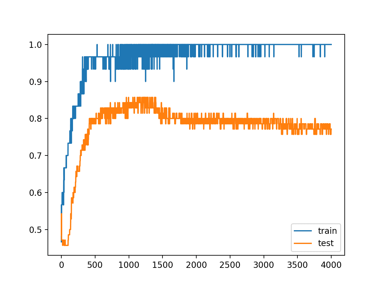
Line Plot of Train and Test Accuracy With Input Layer Noise
MLP With Hidden Layer Noise
An alternative approach to adding noise to the input values is to add noise between the hidden layers.
This can be done by adding noise to the linear output of the layer (weighted sum) before the activation function is applied, in this case a rectified linear activation function. We can also use a larger standard deviation for the noise as the model is less sensitive to noise at this level given the presumably larger weights from being overfit. We will use a standard deviation of 0.1, again, chosen arbitrarily.
# define model
model = Sequential()
model.add(Dense(500, input_dim=2))
model.add(GaussianNoise(0.1))
model.add(Activation('relu'))
model.add(Dense(1, activation='sigmoid'))
model.compile(loss='binary_crossentropy', optimizer='adam', metrics=['accuracy'])
The complete example with Gaussian noise between the hidden layers is listed below.
# mlp overfit on the two circles dataset with hidden layer noise
from sklearn.datasets import make_circles
from keras.models import Sequential
from keras.layers import Dense
from keras.layers import Activation
from keras.layers import GaussianNoise
from matplotlib import pyplot
# generate 2d classification dataset
X, y = make_circles(n_samples=100, noise=0.1, random_state=1)
# split into train and test
n_train = 30
trainX, testX = X[:n_train, :], X[n_train:, :]
trainy, testy = y[:n_train], y[n_train:]
# define model
model = Sequential()
model.add(Dense(500, input_dim=2))
model.add(GaussianNoise(0.1))
model.add(Activation('relu'))
model.add(Dense(1, activation='sigmoid'))
model.compile(loss='binary_crossentropy', optimizer='adam', metrics=['accuracy'])
# fit model
history = model.fit(trainX, trainy, validation_data=(testX, testy), epochs=4000, verbose=0)
# evaluate the model
_, train_acc = model.evaluate(trainX, trainy, verbose=0)
_, test_acc = model.evaluate(testX, testy, verbose=0)
print('Train: %.3f, Test: %.3f' % (train_acc, test_acc))
# plot history
pyplot.plot(history.history['acc'], label='train')
pyplot.plot(history.history['val_acc'], label='test')
pyplot.legend()
pyplot.show()
Running the example reports the model performance on the train and test datasets.
Your results will vary, given both the stochastic nature of the learning algorithm and the stochastic nature of the noise added to the model. Try running the example a few times.
In this case, we can see a marked increase in the performance of the model on the hold out test set.
# Train: 0.967, Test: 0.814
We can also see from the line plot of accuracy over training epochs that the model no longer appears to show the properties of being overfit.
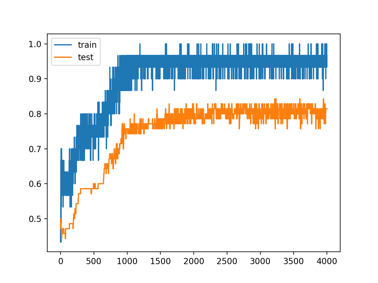
Line Plot of Train and Test Accuracy With Hidden Layer Noise
We can also experiment and add the noise after the outputs of the first hidden layer pass through the activation function.
# define model
model = Sequential()
model.add(Dense(500, input_dim=2, activation='relu'))
model.add(GaussianNoise(0.1))
model.add(Dense(1, activation='sigmoid'))
model.compile(loss='binary_crossentropy', optimizer='adam', metrics=['accuracy'])
The complete example is listed below.
# mlp overfit on the two circles dataset with hidden layer noise (alternate)
from sklearn.datasets import make_circles
from keras.models import Sequential
from keras.layers import Dense
from keras.layers import GaussianNoise
from matplotlib import pyplot
# generate 2d classification dataset
X, y = make_circles(n_samples=100, noise=0.1, random_state=1)
# split into train and test
n_train = 30
trainX, testX = X[:n_train, :], X[n_train:, :]
trainy, testy = y[:n_train], y[n_train:]
# define model
model = Sequential()
model.add(Dense(500, input_dim=2, activation='relu'))
model.add(GaussianNoise(0.1))
model.add(Dense(1, activation='sigmoid'))
model.compile(loss='binary_crossentropy', optimizer='adam', metrics=['accuracy'])
# fit model
history = model.fit(trainX, trainy, validation_data=(testX, testy), epochs=4000, verbose=0)
# evaluate the model
_, train_acc = model.evaluate(trainX, trainy, verbose=0)
_, test_acc = model.evaluate(testX, testy, verbose=0)
print('Train: %.3f, Test: %.3f' % (train_acc, test_acc))
# plot history
pyplot.plot(history.history['acc'], label='train')
pyplot.plot(history.history['val_acc'], label='test')
pyplot.legend()
pyplot.show()
Running the example reports the model performance on the train and test datasets.
Surprisingly, we see little difference in the performance of the model.
Train: 0.967, Test: 0.814
Again, we can see from the line plot of accuracy over training epochs that the model no longer shows sign of overfitting.
Line Plot of Train and Test Accuracy With Hidden Layer Noise (alternate)
Extensions
This section lists some ideas for extending the tutorial that you may wish to explore.
- Repeated Evaluation. Update the example to use repeated evaluation of the model with and without noise and report performance as the mean and standard deviation over repeats.
- Grid Search Standard Deviation. Develop a grid search in order to discover the amount of noise that reliably results in the best performing model.
- Input and Hidden Noise. Update the example to introduce noise at both the input and hidden layers of the model.
If you explore any of these extensions, I’d love to know.
Further Reading
This section provides more resources on the topic if you are looking to go deeper.
- Keras Regularizers API
- Keras Core Layers API
- Keras Convolutional Layers API
- Keras Recurrent Layers API
- Keras Noise API
- sklearn.datasets.make_circles API
Summary
In this tutorial, you discovered how to add noise to deep learning models in Keras in order to reduce overfitting and improve model generalization.
Specifically, you learned:
- Noise can be added to a neural network model via the GaussianNoise layer.
- The GaussianNoise can be used to add noise to input values or between hidden layers.
- How to add a GaussianNoise layer in order to reduce overfitting in a Multilayer Perceptron model for classification.
Do you have any questions?
Ask your questions in the comments below and I will do my best to answer.
The post How to Improve Deep Learning Model Robustness by Adding Noise appeared first on Machine Learning Mastery.