Author: Jason Brownlee
Deep learning neural network models are highly flexible nonlinear algorithms capable of learning a near infinite number of mapping functions.
A frustration with this flexibility is the high variance in a final model. The same neural network model trained on the same dataset may find one of many different possible “good enough” solutions each time it is run.
Model averaging is an ensemble learning technique that reduces the variance in a final neural network model, sacrificing spread in the performance of the model for a confidence in what performance to expect from the model.
In this tutorial, you will discover how to develop a model averaging ensemble in Keras to reduce the variance in a final model.
After completing this tutorial, you will know:
- Model averaging is an ensemble learning technique that can be used to reduce the expected variance of deep learning neural network models.
- How to implement model averaging in Keras for classification and regression predictive modeling problems.
- How to work through a multi-class classification problem and use model averaging to reduce the variance of the final model.
Let’s get started.
How to Reduce the Variance of Deep Learning Models in Keras With Model Averaging Ensembles
Photo by John Mason, some rights reserved.
Tutorial Overview
This tutorial is divided into six parts; they are:
- Model Averaging
- How to Average Models in Keras
- Multi-Class Classification Problem
- MLP Model for Multi-Class Classification
- High Variance of MLP Model
- Model Averaging Ensemble
Model Averaging
Deep learning neural network models are nonlinear methods that learn via a stochastic training algorithm.
This means that they are highly flexible, capable of learning complex relationships between variables and approximating any mapping function, given enough resources. A downside of this flexibility is that the models suffer high variance.
This means that the models are highly dependent on the specific training data used to train the model and on the initial conditions (random initial weights) and serendipity during the training process. The result is a final model that makes different predictions each time the same model configuration is trained on the same dataset.
This can be frustrating when training a final model for use in making predictions on new data, such as operationally or in a machine learning competition.
The high variance of the approach can be addressed by training multiple models for the problem and combining their predictions. This approach is called model averaging and belongs to a family of techniques called ensemble learning.
Want Better Results with Deep Learning?
Take my free 7-day email crash course now (with sample code).
Click to sign-up and also get a free PDF Ebook version of the course.
How to Average Models in Keras
The simplest way to develop a model averaging ensemble in Keras is to train multiple models on the same dataset then combine the predictions from each of the trained models.
Train Multiple Models
Training multiple models may be resource intensive, depending on the size of the model and the size of the training data.
You may have to train the models sequentially on the same hardware. For very large models, it may be worth training the models in parallel using cloud infrastructure such as Amazon Web Services.
The number of models required for the ensemble may vary based on the complexity of the problem and model. A benefit of the approach is that you can continue to create models, add them to the ensemble, and evaluate their impact on the performance by making predictions on a holdout test set.
For small models, you can train the models sequentially and keep them in memory for use in your experiment. For example:
...
# train models and keep them in memory
n_members = 10
models = list()
for _ in range(n_members):
	# define and fit model
	model = ...
	# store model in memory as ensemble member
	models.add(models)
...
For large models, perhaps trained on different hardware, you can save each model to file.
...
# train models and keep them to file
n_members = 10
for i in range(n_members):
	# define and fit model
	model = ...
	# save model to file
	filename = 'model_' + str(i + 1) + '.h5'
	model.save(filename)
	print('Saved: %s' % filename)
...
Models can then be loaded later.
Small models can all be loaded into memory at the same time, whereas very large models may have to be loaded one at a time to make a prediction, then later to have the predictions combined.
from keras.models import load_model
...
# load pre-trained ensemble members
n_members = 10
models = list()
for i in range(n_members):
	# load model
	filename = 'model_' + str(i + 1) + '.h5'
	model = load_model(filename)
	# store in memory
	models.append(model)
...
Combine Predictions
Once the models have been prepared, each model can be used to make a prediction and the predictions can be combined.
In the case of a regression problem where each model is predicting a real-valued output, the values can be collected and the average calculated.
...
# make predictions
yhats = [model.predict(testX) for model in models]
yhats = array(yhats)
# calculate average
outcomes = mean(yhats)
In the case of a classification problem, there are two options.
The first is to calculate the mode of the predicted integer class values.
...
# make predictions
yhats = [model.predict_classes(testX) for model in models]
yhats = array(yhats)
# calculate mode
outcomes, _ = mode(yhats)
A downside of this approach is that for small ensembles or problems with a large number of classes, the sample of predictions may not be large enough for the mode to be meaningful.
In the case of a binary classification problem, a sigmoid activation function is used on the output layer and the average of the predicted probabilities can be calculated much like a regression problem.
In the case of a multi-class classification problem with more than two classes, a softmax activation function is used on the output layer and the sum of the probabilities for each predicted class can be calculated before taking the argmax to get the class value.
...
# make predictions
yhats = [model.predict(testX) for model in models]
yhats = array(yhats)
# sum across ensembles
summed = numpy.sum(yhats, axis=0)
# argmax across classes
outcomes = argmax(summed, axis=1)
These approaches for combining predictions of Keras models will work just as well for Multilayer Perceptron, Convolutional, and Recurrent Neural Networks.
Now that we know how to average predictions from multiple neural network models in Keras, let’s work through a case study.
Multi-Class Classification Problem
We will use a small multi-class classification problem as the basis to demonstrate a model averaging ensemble.
The scikit-learn class provides the make_blobs() function that can be used to create a multi-class classification problem with the prescribed number of samples, input variables, classes, and variance of samples within a class.
We use this problem with 500 examples, with input variables (to represent the x and y coordinates of the points) and a standard deviation of 2.0 for points within each group. We will use the same random state (seed for the pseudorandom number generator) to ensure that we always get the same 500 points.
# generate 2d classification dataset
X, y = make_blobs(n_samples=500, centers=3, n_features=2, cluster_std=2, random_state=2)
The results are the input and output elements of a dataset that we can model.
In order to get a feeling for the complexity of the problem, we can graph each point on a two-dimensional scatter plot and color each point by class value.
The complete example is listed below.
# scatter plot of blobs dataset
from sklearn.datasets.samples_generator import make_blobs
from matplotlib import pyplot
from pandas import DataFrame
# generate 2d classification dataset
X, y = make_blobs(n_samples=500, centers=3, n_features=2, cluster_std=2, random_state=2)
# scatter plot, dots colored by class value
df = DataFrame(dict(x=X[:,0], y=X[:,1], label=y))
colors = {0:'red', 1:'blue', 2:'green'}
fig, ax = pyplot.subplots()
grouped = df.groupby('label')
for key, group in grouped:
    group.plot(ax=ax, kind='scatter', x='x', y='y', label=key, color=colors[key])
pyplot.show()
Running the example creates a scatter plot of the entire dataset. We can see that the standard deviation of 2.0 means that the classes are not linearly separable (separable by a line) causing many ambiguous points.
This is desirable as it means that the problem is non-trivial and will allow a neural network model to find many different “good enough” candidate solutions resulting in a high variance.
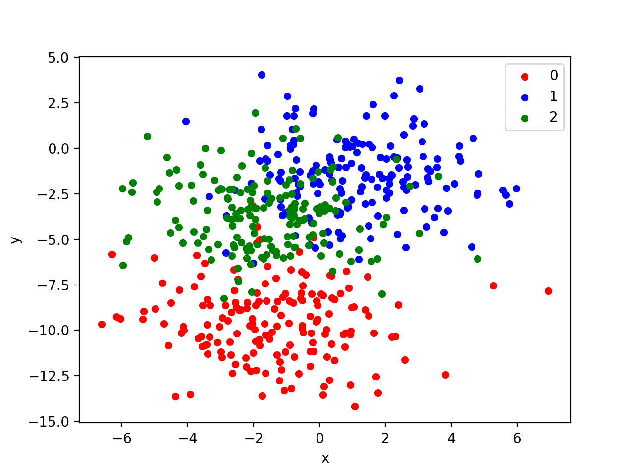
Scatter Plot of Blobs Dataset with Three Classes and Points Colored by Class Value
MLP Model for Multi-Class Classification
Now that we have defined a problem, we can define a model to address it.
We will define a model that is perhaps under-constrained and not tuned to the problem. This is intentional to demonstrate the high variance of a neural network model seen on truly large and challenging supervised learning problems.
The problem is a multi-class classification problem, and we will model it using a softmax activation function on the output layer. This means that the model will predict a vector with 3 elements with the probability that the sample belongs to each of the 3 classes. Therefore, the first step is to one hot encode the class values.
y = to_categorical(y)
Next, we must split the dataset into training and test sets. We will use the test set both to evaluate the performance of the model and to plot its performance during training with a learning curve. We will use 30% of the data for training and 70% for the test set.
This is an example of a challenging problem where we have more unlabeled examples than we do labeled examples.
# split into train and test
n_train = int(0.3 * X.shape[0])
trainX, testX = X[:n_train, :], X[n_train:, :]
trainy, testy = y[:n_train], y[n_train:]
Next, we can define and compile the model.
The model will expect samples with two input variables. The model then has a single hidden layer with 15 modes and a rectified linear activation function, then an output layer with 3 nodes to predict the probability of each of the 3 classes and a softmax activation function.
Because the problem is multi-class, we will use the categorical cross entropy loss function to optimize the model and the efficient Adam flavor of stochastic gradient descent.
# define model
model = Sequential()
model.add(Dense(15, input_dim=2, activation='relu'))
model.add(Dense(3, activation='softmax'))
model.compile(loss='categorical_crossentropy', optimizer='adam', metrics=['accuracy'])
The model is fit for 200 training epochs and we will evaluate the model each epoch on the test set, using the test set as a validation set.
# fit model
history = model.fit(trainX, trainy, validation_data=(testX, testy), epochs=200, verbose=0)
At the end of the run, we will evaluate the performance of the model on both the train and the test sets.
# evaluate the model
_, train_acc = model.evaluate(trainX, trainy, verbose=0)
_, test_acc = model.evaluate(testX, testy, verbose=0)
print('Train: %.3f, Test: %.3f' % (train_acc, test_acc))
Then finally, we will plot learning curves of the model accuracy over each training epoch on both the training and test dataset.
# plot history
pyplot.plot(history.history['acc'], label='train')
pyplot.plot(history.history['val_acc'], label='test')
pyplot.legend()
pyplot.show()
The complete example is listed below.
# fit high variance mlp on blobs classification problem
from sklearn.datasets.samples_generator import make_blobs
from keras.utils import to_categorical
from keras.models import Sequential
from keras.layers import Dense
from matplotlib import pyplot
# generate 2d classification dataset
X, y = make_blobs(n_samples=500, centers=3, n_features=2, cluster_std=2, random_state=2)
y = to_categorical(y)
# split into train and test
n_train = int(0.3 * X.shape[0])
trainX, testX = X[:n_train, :], X[n_train:, :]
trainy, testy = y[:n_train], y[n_train:]
# define model
model = Sequential()
model.add(Dense(15, input_dim=2, activation='relu'))
model.add(Dense(3, activation='softmax'))
model.compile(loss='categorical_crossentropy', optimizer='adam', metrics=['accuracy'])
# fit model
history = model.fit(trainX, trainy, validation_data=(testX, testy), epochs=200, verbose=0)
# evaluate the model
_, train_acc = model.evaluate(trainX, trainy, verbose=0)
_, test_acc = model.evaluate(testX, testy, verbose=0)
print('Train: %.3f, Test: %.3f' % (train_acc, test_acc))
# learning curves of model accuracy
pyplot.plot(history.history['acc'], label='train')
pyplot.plot(history.history['val_acc'], label='test')
pyplot.legend()
pyplot.show()
Running the example first prints the performance of the final model on the train and test datasets.
Your specific results will vary (by design!) given the high variance nature of the model.
In this case, we can see that the model achieved about 84% accuracy on the training dataset and about 76% accuracy on the test dataset; not terrible.
Train: 0.847, Test: 0.766
A line plot is also created showing the learning curves for the model accuracy on the train and test sets over each training epoch.
We can see that the model is not really overfit, but is perhaps a little underfit and may benefit from an increase in capacity, more training, and perhaps some regularization. All of these improvements of which we intentionally hold back to force the high variance for our case study.
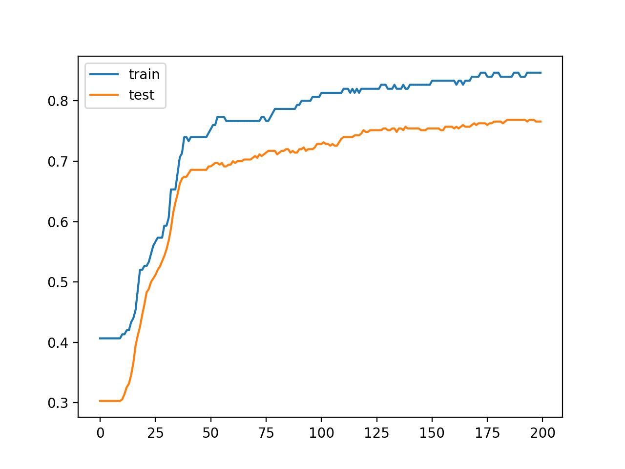
Line Plot Learning Curves of Model Accuracy on Train and Test Dataset Over Each Training Epoch
High Variance of MLP Model
It is important to demonstrate that the model indeed has a variance in its prediction.
We can demonstrate this by repeating the fit and evaluation of the same model configuration on the same dataset and summarizing the final performance of the model.
To do this, we first split the fit and evaluation of the model out as a function that we can call repeatedly. The evaluate_model() function below takes the train and test dataset, fits a model, then evaluates it, retuning the accuracy of the model on the test dataset.
# fit and evaluate a neural net model on the dataset
def evaluate_model(trainX, trainy, testX, testy):
	# define model
	model = Sequential()
	model.add(Dense(15, input_dim=2, activation='relu'))
	model.add(Dense(3, activation='softmax'))
	model.compile(loss='categorical_crossentropy', optimizer='adam', metrics=['accuracy'])
	# fit model
	model.fit(trainX, trainy, epochs=200, verbose=0)
	# evaluate the model
	_, test_acc = model.evaluate(testX, testy, verbose=0)
	return test_acc
We can call this function 30 times, saving the test accuracy scores.
# repeated evaluation
n_repeats = 30
scores = list()
for _ in range(n_repeats):
	score = evaluate_model(trainX, trainy, testX, testy)
	print('> %.3f' % score)
	scores.append(score)
Once collected, we can summarize the distribution scores, first in terms of the mean and standard deviation, assuming the distribution is Gaussian, which is very reasonable.
# summarize the distribution of scores
print('Scores Mean: %.3f, Standard Deviation: %.3f' % (mean(scores), std(scores)))
We can then summarize the distribution both as a histogram to show the shape of the distribution and as a box and whisker plot to show the spread and body of the distribution.
# histogram of distribution
pyplot.hist(scores, bins=10)
pyplot.show()
# boxplot of distribution
pyplot.boxplot(scores)
pyplot.show()
The complete example of summarizing the variance of the MLP model on the chosen blobs dataset is listed below.
# demonstrate high variance of mlp model on blobs classification problem
from sklearn.datasets.samples_generator import make_blobs
from keras.utils import to_categorical
from keras.models import Sequential
from keras.layers import Dense
from numpy import mean
from numpy import std
from matplotlib import pyplot

# fit and evaluate a neural net model on the dataset
def evaluate_model(trainX, trainy, testX, testy):
	# define model
	model = Sequential()
	model.add(Dense(15, input_dim=2, activation='relu'))
	model.add(Dense(3, activation='softmax'))
	model.compile(loss='categorical_crossentropy', optimizer='adam', metrics=['accuracy'])
	# fit model
	model.fit(trainX, trainy, epochs=200, verbose=0)
	# evaluate the model
	_, test_acc = model.evaluate(testX, testy, verbose=0)
	return test_acc

# generate 2d classification dataset
X, y = make_blobs(n_samples=500, centers=3, n_features=2, cluster_std=2, random_state=2)
y = to_categorical(y)
# split into train and test
n_train = int(0.3 * X.shape[0])
trainX, testX = X[:n_train, :], X[n_train:, :]
trainy, testy = y[:n_train], y[n_train:]
# repeated evaluation
n_repeats = 30
scores = list()
for _ in range(n_repeats):
	score = evaluate_model(trainX, trainy, testX, testy)
	print('> %.3f' % score)
	scores.append(score)
# summarize the distribution of scores
print('Scores Mean: %.3f, Standard Deviation: %.3f' % (mean(scores), std(scores)))
# histogram of distribution
pyplot.hist(scores, bins=10)
pyplot.show()
# boxplot of distribution
pyplot.boxplot(scores)
pyplot.show()
Running the example first prints the accuracy of each model on the test set, finishing with the mean and standard deviation of the sample of accuracy scores.
The specifics of your sample may differ, but the summary statistics should be similar.
In this case, we can see that the average of the sample is 77% with a standard deviation of about 1.4%. Assuming a Gaussian distribution, we would expect 99% of accuracy scores to fall between about 73% and 81% (i.e. 3 standard deviations above and below the mean).
We can take the standard deviation of the accuracy of the model on the test set as an estimate for the variance of the predictions made by the model.
> 0.749
> 0.771
> 0.763
> 0.760
> 0.783
> 0.780
> 0.769
> 0.754
> 0.766
> 0.786
> 0.766
> 0.774
> 0.757
> 0.754
> 0.771
> 0.749
> 0.763
> 0.800
> 0.774
> 0.777
> 0.766
> 0.794
> 0.797
> 0.757
> 0.763
> 0.751
> 0.789
> 0.791
> 0.766
> 0.766
Scores Mean: 0.770, Standard Deviation: 0.014
A histogram of the accuracy scores is also created, showing a very rough Gaussian shape, perhaps with a longer right tail.
A large sample and a different number of bins on the plot might better expose the true underlying shape of the distribution.
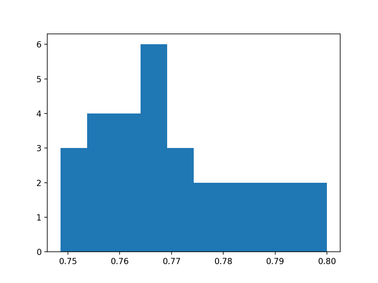
Histogram of Model Test Accuracy Over 30 Repeats
A box and whisker plot is also created showing a line at the median at about 76.5% accuracy on the test set and the interquartile range or middle 50% of the samples between about 78% and 76%.
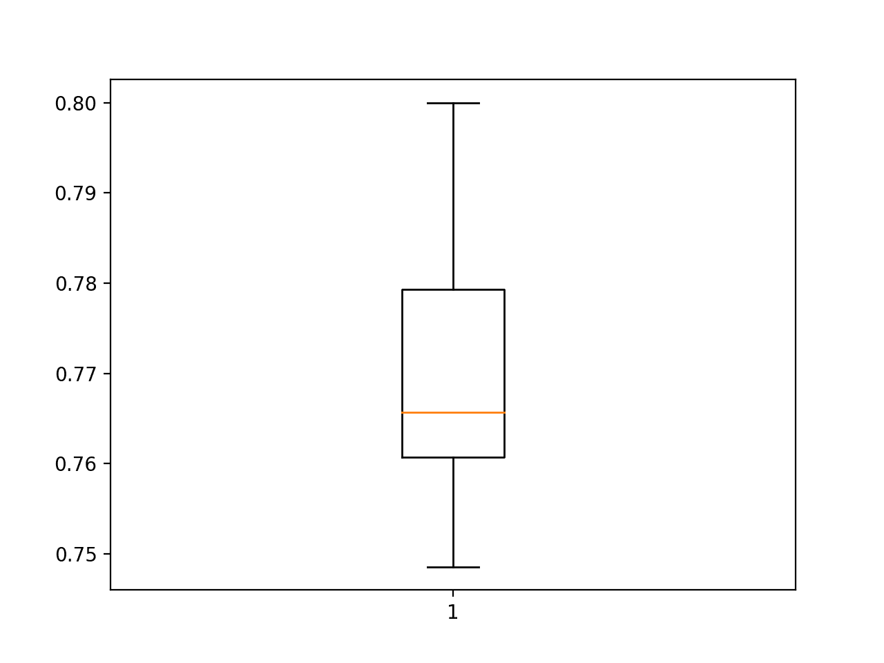
Box and Whisker Plot of Model Test Accuracy Over 30 Repeats
The analysis of the sample of test scores clearly demonstrates a variance in the performance of the same model trained on the same dataset.
A spread of likely scores of about 8 percentage points (81% – 73%) on the test set could reasonably be considered large, e.g. a high variance result.
Model Averaging Ensemble
We can use model averaging to both reduce the variance of the model and possibly reduce the generalization error of the model.
Specifically, this would result in a smaller standard deviation on the holdout test set and a better performance on the training set. We can check both of these assumptions.
First, we must develop a function to prepare and return a fit model on the training dataset.
# fit model on dataset
def fit_model(trainX, trainy):
	# define model
	model = Sequential()
	model.add(Dense(15, input_dim=2, activation='relu'))
	model.add(Dense(3, activation='softmax'))
	model.compile(loss='categorical_crossentropy', optimizer='adam', metrics=['accuracy'])
	# fit model
	model.fit(trainX, trainy, epochs=200, verbose=0)
	return model
Next, we need a function that can take a list of ensemble members and make a prediction for an out of sample dataset. This could be one or more samples arranged in a two-dimensional array of samples and input features.
Hint: you can use this function yourself for testing ensembles and for making predictions with ensembles on new data.
# make an ensemble prediction for multi-class classification
def ensemble_predictions(members, testX):
	# make predictions
	yhats = [model.predict(testX) for model in members]
	yhats = array(yhats)
	# sum across ensemble members
	summed = numpy.sum(yhats, axis=0)
	# argmax across classes
	result = argmax(summed, axis=1)
	return result
We don’t know how many ensemble members will be appropriate for this problem.
Therefore, we can perform a sensitivity analysis of the number of ensemble members and how it impacts test accuracy. This means we need a function that can evaluate a specified number of ensemble members and return the accuracy of a prediction combined from those members.
# evaluate a specific number of members in an ensemble
def evaluate_n_members(members, n_members, testX, testy):
	# select a subset of members
	subset = members[:n_members]
	print(len(subset))
	# make prediction
	yhat = ensemble_predictions(subset, testX)
	# calculate accuracy
	return accuracy_score(testy, yhat)
Finally, we can create a line plot of the number of ensemble members (x-axis) versus the accuracy of a prediction averaged across that many members on the test dataset (y-axis).
# plot score vs number of ensemble members
x_axis = [i for i in range(1, n_members+1)]
pyplot.plot(x_axis, scores)
pyplot.show()
The complete example is listed below.
# model averaging ensemble and a study of ensemble size on test accuracy
from sklearn.datasets.samples_generator import make_blobs
from keras.utils import to_categorical
from keras.models import Sequential
from keras.layers import Dense
import numpy
from numpy import array
from numpy import argmax
from sklearn.metrics import accuracy_score
from matplotlib import pyplot

# fit model on dataset
def fit_model(trainX, trainy):
	# define model
	model = Sequential()
	model.add(Dense(15, input_dim=2, activation='relu'))
	model.add(Dense(3, activation='softmax'))
	model.compile(loss='categorical_crossentropy', optimizer='adam', metrics=['accuracy'])
	# fit model
	model.fit(trainX, trainy, epochs=200, verbose=0)
	return model

# make an ensemble prediction for multi-class classification
def ensemble_predictions(members, testX):
	# make predictions
	yhats = [model.predict(testX) for model in members]
	yhats = array(yhats)
	# sum across ensemble members
	summed = numpy.sum(yhats, axis=0)
	# argmax across classes
	result = argmax(summed, axis=1)
	return result

# evaluate a specific number of members in an ensemble
def evaluate_n_members(members, n_members, testX, testy):
	# select a subset of members
	subset = members[:n_members]
	print(len(subset))
	# make prediction
	yhat = ensemble_predictions(subset, testX)
	# calculate accuracy
	return accuracy_score(testy, yhat)

# generate 2d classification dataset
X, y = make_blobs(n_samples=500, centers=3, n_features=2, cluster_std=2, random_state=2)
# split into train and test
n_train = int(0.3 * X.shape[0])
trainX, testX = X[:n_train, :], X[n_train:, :]
trainy, testy = y[:n_train], y[n_train:]
trainy = to_categorical(trainy)
# fit all models
n_members = 20
members = [fit_model(trainX, trainy) for _ in range(n_members)]
# evaluate different numbers of ensembles
scores = list()
for i in range(1, n_members+1):
	score = evaluate_n_members(members, i, testX, testy)
	print('> %.3f' % score)
	scores.append(score)
# plot score vs number of ensemble members
x_axis = [i for i in range(1, n_members+1)]
pyplot.plot(x_axis, scores)
pyplot.show()
Running the example first fits 20 models on the same training dataset, which may take less than a minute on modern hardware.
Then, different sized ensembles are tested from 1 member to all 20 members and test accuracy results are printed for each ensemble size.
1
> 0.740
2
> 0.754
3
> 0.754
4
> 0.760
5
> 0.763
6
> 0.763
7
> 0.763
8
> 0.763
9
> 0.760
10
> 0.760
11
> 0.763
12
> 0.763
13
> 0.766
14
> 0.763
15
> 0.760
16
> 0.760
17
> 0.763
18
> 0.766
19
> 0.763
20
> 0.763
Finally, a line plot is created showing the relationship between ensemble size and performance on the test set.
We can see that performance improves to about five members, after which performance plateaus around 76% accuracy. This is close to the average test set performance observed during the analysis of the repeated evaluation of the model.
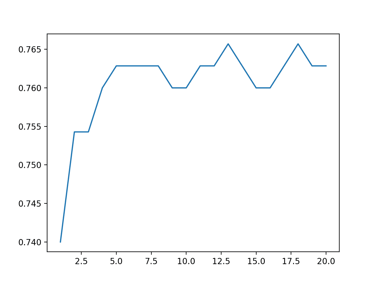
Line Plot of Ensemble Size Versus Model Test Accuracy
Finally, we can update the repeated evaluation experiment to use an ensemble of five models instead of a single model and compare the distribution of scores.
The complete example of a repeated evaluated five-member ensemble of the blobs dataset is listed below.
# repeated evaluation of model averaging ensemble on blobs dataset
from sklearn.datasets.samples_generator import make_blobs
from keras.utils import to_categorical
from keras.models import Sequential
from keras.layers import Dense
import numpy
from numpy import array
from numpy import argmax
from numpy import mean
from numpy import std
from sklearn.metrics import accuracy_score

# fit model on dataset
def fit_model(trainX, trainy):
	# define model
	model = Sequential()
	model.add(Dense(15, input_dim=2, activation='relu'))
	model.add(Dense(3, activation='softmax'))
	model.compile(loss='categorical_crossentropy', optimizer='adam', metrics=['accuracy'])
	# fit model
	model.fit(trainX, trainy, epochs=200, verbose=0)
	return model

# make an ensemble prediction for multi-class classification
def ensemble_predictions(members, testX):
	# make predictions
	yhats = [model.predict(testX) for model in members]
	yhats = array(yhats)
	# sum across ensemble members
	summed = numpy.sum(yhats, axis=0)
	# argmax across classes
	result = argmax(summed, axis=1)
	return result

# evaluate ensemble model
def evaluate_members(members, testX, testy):
	# make prediction
	yhat = ensemble_predictions(members, testX)
	# calculate accuracy
	return accuracy_score(testy, yhat)

# generate 2d classification dataset
X, y = make_blobs(n_samples=500, centers=3, n_features=2, cluster_std=2, random_state=2)
# split into train and test
n_train = int(0.3 * X.shape[0])
trainX, testX = X[:n_train, :], X[n_train:, :]
trainy, testy = y[:n_train], y[n_train:]
trainy = to_categorical(trainy)
# repeated evaluation
n_repeats = 30
n_members = 5
scores = list()
for _ in range(n_repeats):
	# fit all models
	members = [fit_model(trainX, trainy) for _ in range(n_members)]
	# evaluate ensemble
	score = evaluate_members(members, testX, testy)
	print('> %.3f' % score)
	scores.append(score)
# summarize the distribution of scores
print('Scores Mean: %.3f, Standard Deviation: %.3f' % (mean(scores), std(scores)))
Running the example may take a few minutes as five models are fit and evaluated and this process is repeated 30 times.
The performance of each model on the test set is printed to provide an indication of progress.
The mean and standard deviation of the model performance is printed at the end of the run. Your specific results may vary, but not by much.
> 0.769
> 0.757
> 0.754
> 0.780
> 0.771
> 0.774
> 0.766
> 0.769
> 0.774
> 0.771
> 0.760
> 0.766
> 0.766
> 0.769
> 0.766
> 0.771
> 0.763
> 0.760
> 0.771
> 0.780
> 0.769
> 0.757
> 0.769
> 0.771
> 0.771
> 0.766
> 0.763
> 0.766
> 0.771
> 0.769
Scores Mean: 0.768, Standard Deviation: 0.006
In this case, we can see that the average performance of a five-member ensemble on the dataset is 76%. This is very close to the average of 77% seen for a single model.
The important difference is the standard deviation shrinking from 1.4% for a single model to 0.6% with an ensemble of five models. We might expect that a given ensemble of five models on this problem to have a performance fall between about 74% and about 78% with a likelihood of 99%.
Averaging the same model trained on the same dataset gives us a spread for improved reliability, a property often highly desired in a final model to be used operationally.
More models in the ensemble will further decrease the standard deviation of the accuracy of an ensemble on the test dataset given the law of large numbers, at least to a point of diminishing returns.
This demonstrates that for this specific model and prediction problem, that a model averaging ensemble with five members is sufficient to reduce the variance of the model. This reduction in variance, in turn, also means a better on-average performance when preparing a final model.
Extensions
This section lists some ideas for extending the tutorial that you may wish to explore.
- Average Class Prediction. Update the example to average the class integer prediction instead of the class probability prediction and compare results.
- Save and Load Models. Update the example to save ensemble members to file, then load them from a separate script for evaluation.
- Sensitivity of Variance. Create a new example that performs a sensitivity analysis of the number of ensemble members on the standard deviation of model performance on the test set over a given number of repeats and report the point of diminishing returns.
If you explore any of these extensions, I’d love to know.
Further Reading
This section provides more resources on the topic if you are looking to go deeper.
- Getting started with the Keras Sequential model
- Keras Core Layers API
- scipy.stats.mode API
- numpy.argmax API
- sklearn.datasets.make_blobs API
Summary
In this tutorial, you discovered how to develop a model averaging ensemble in Keras to reduce the variance in a final model.
Specifically, you learned:
- Model averaging is an ensemble learning technique that can be used to reduce the expected variance of deep learning neural network models.
- How to implement model averaging in Keras for classification and regression predictive modeling problems.
- How to work through a multi-class classification problem and use model averaging to reduce the variance of the final model.
Do you have any questions?
Ask your questions in the comments below and I will do my best to answer.
The post How to Reduce the Variance of Deep Learning Models in Keras Using Model Averaging Ensembles appeared first on Machine Learning Mastery.