
Author: Jason Brownlee
Ensemble learning are methods that combine the predictions from multiple models.
It is important in ensemble learning that the models that comprise the ensemble are good, making different prediction errors. Predictions that are good in different ways can result in a prediction that is both more stable and often better than the predictions of any individual member model.
One way to achieve differences between models is to train each model on a different subset of the available training data. Models are trained on different subsets of the training data naturally through the use of resampling methods such as cross-validation and the bootstrap, designed to estimate the average performance of the model generally on unseen data. The models used in this estimation process can be combined in what is referred to as a resampling-based ensemble, such as a cross-validation ensemble or a bootstrap aggregation (or bagging) ensemble.
In this tutorial, you will discover how to develop a suite of different resampling-based ensembles for deep learning neural network models.
After completing this tutorial, you will know:
- How to estimate model performance using random-splits and develop an ensemble from the models.
- How to estimate performance using 10-fold cross-validation and develop a cross-validation ensemble.
- How to estimate performance using the bootstrap and combine models using a bagging ensemble.
Let’s get started.

How to Create a Random-Split, Cross-Validation, and Bagging Ensembles for Deep Learning in Keras
Photo by Gian Luca Ponti, some rights reserved.
Tutorial Overview
This tutorial is divided into six parts; they are:
- Data Resampling Ensembles
- Multi-Class Classification Problem
- Single Multilayer Perceptron Model
- Random Splits Ensemble
- Cross-Validation Ensemble
- Bagging Ensemble Ensemble
Data Resampling Ensembles
Combining the predictions from multiple models can result in more stable predictions, and in some cases, predictions that have better performance than any of the contributing models.
Effective ensembles require members that disagree. Each member must have skill (e.g. perform better than random chance), but ideally, perform well in different ways. Technically, we can say that we prefer ensemble members to have low correlation in their predictions, or prediction errors.
One approach to encourage differences between ensembles is to use the same learning algorithm on different training datasets. This can be achieved by repeatedly resampling a training dataset that is in turn used to train a new model. Multiple models are fit using slightly different perspectives on the training data and, in turn, make different errors and often more stable and better predictions when combined.
We can refer to these methods generally as data resampling ensembles.
A benefit of this approach is that resampling methods may be used that do not make use of all examples in the training dataset. Any examples that are not used to fit the model can be used as a test dataset to estimate the generalization error of the chosen model configuration.
There are three popular resampling methods that we could use to create a resampling ensemble; they are:
- Random Splits. The dataset is repeatedly sampled with a random split of the data into train and test sets.
- k-fold Cross-Validation. The dataset is split into k equally sized folds, k models are trained and each fold is given an opportunity to be used as the holdout set where the model is trained on all remaining folds.
- Bootstrap Aggregation. Random samples are collected with replacement and examples not included in a given sample are used as the test set.
Perhaps the most widely used resampling ensemble method is bootstrap aggregation, more commonly referred to as bagging. The resampling with replacement allows more difference in the training dataset, biasing the model and, in turn, resulting in more difference between the predictions of the resulting models.
Resampling ensemble models makes some specific assumptions about your project:
- That a robust estimate of model performance on unseen data is required; if not, then a single train/test split can be used.
- That there is a potential for a lift in performance using an ensemble of models; if not, then a single model fit on all available data can be used.
- That the computational cost of fitting more than one neural network model on a sample of the training dataset is not prohibitive; if not, all resources should be put into fitting a single model.
Neural network models are remarkably flexible, therefore the lift in performance provided by a resampling ensemble is not always possible given that individual models trained on all available data can perform so well.
As such, the sweet spot for using a resampling ensemble is the case where there is a requirement for a robust estimate of performance and multiple models can be fit to calculate the estimate, but there is also a requirement for one (or more) of the models created during the estimate of performance to be used as the final model (e.g. a new final model cannot be fit on all available training data).
Now that we are familiar with resampling ensemble methods, we can work through an example of applying each method in turn.
Want Better Results with Deep Learning?
Take my free 7-day email crash course now (with sample code).
Click to sign-up and also get a free PDF Ebook version of the course.
Multi-Class Classification Problem
We will use a small multi-class classification problem as the basis to demonstrate a model resampling ensembles.
The scikit-learn class provides the make_blobs() function that can be used to create a multi-class classification problem with the prescribed number of samples, input variables, classes, and variance of samples within a class.
We use this problem with 1,000 examples, with input variables (to represent the x and y coordinates of the points) and a standard deviation of 2.0 for points within each group. We will use the same random state (seed for the pseudorandom number generator) to ensure that we always get the same 1,000 points.
# generate 2d classification dataset
X, y = make_blobs(n_samples=1000, centers=3, n_features=2, cluster_std=2, random_state=2)
The results are the input and output elements of a dataset that we can model.
In order to get a feeling for the complexity of the problem, we can plot each point on a two-dimensional scatter plot and color each point by class value.
The complete example is listed below.
# scatter plot of blobs dataset
from sklearn.datasets.samples_generator import make_blobs
from matplotlib import pyplot
from pandas import DataFrame
# generate 2d classification dataset
X, y = make_blobs(n_samples=1000, centers=3, n_features=2, cluster_std=2, random_state=2)
# scatter plot, dots colored by class value
df = DataFrame(dict(x=X[:,0], y=X[:,1], label=y))
colors = {0:'red', 1:'blue', 2:'green'}
fig, ax = pyplot.subplots()
grouped = df.groupby('label')
for key, group in grouped:
    group.plot(ax=ax, kind='scatter', x='x', y='y', label=key, color=colors[key])
pyplot.show()
Running the example creates a scatter plot of the entire dataset. We can see that the standard deviation of 2.0 means that the classes are not linearly separable (separable by a line) causing many ambiguous points.
This is desirable as it means that the problem is non-trivial and will allow a neural network model to find many different “good enough” candidate solutions resulting in a high variance.
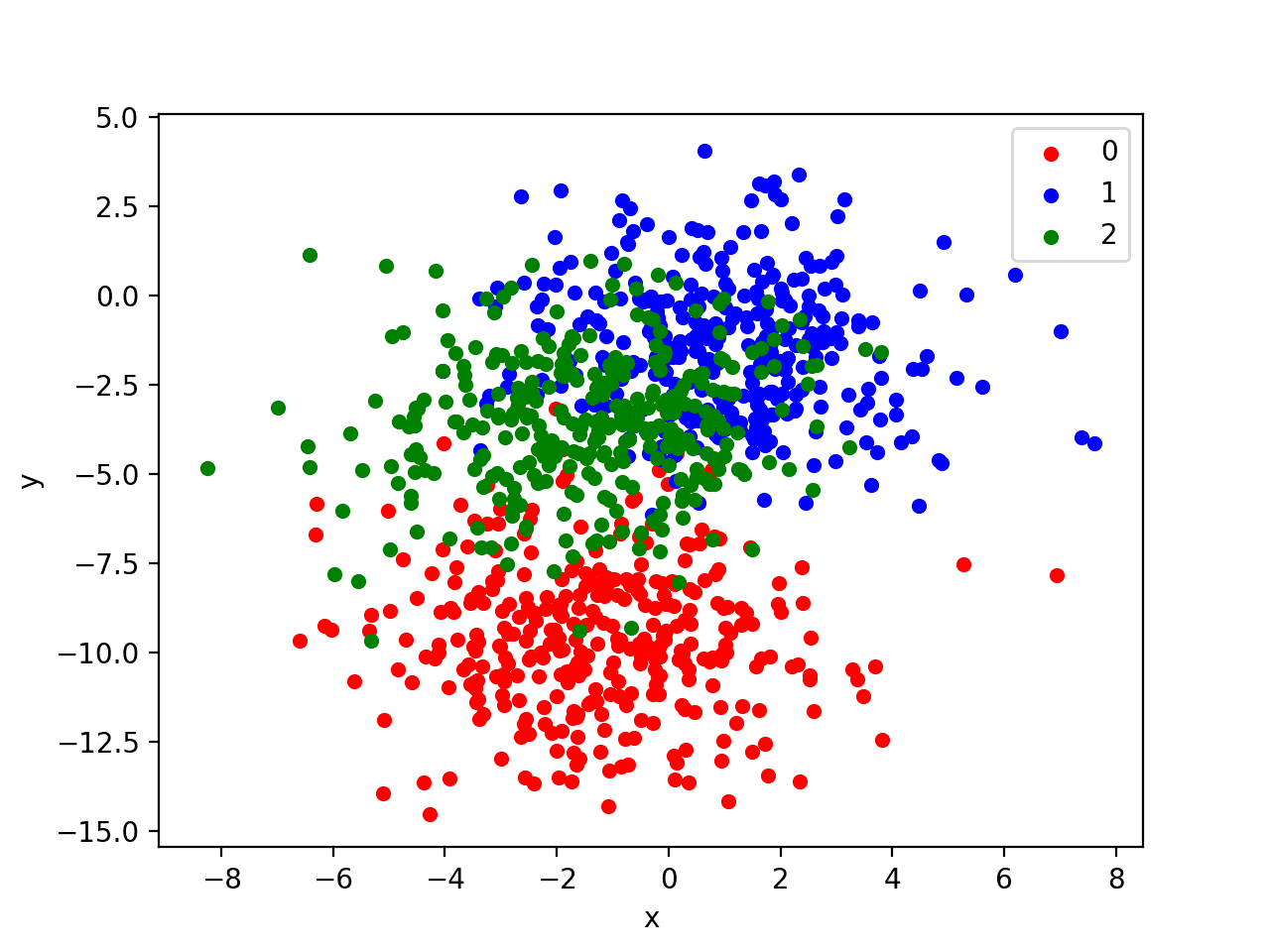
Scatter Plot of Blobs Dataset with Three Classes and Points Colored by Class Value
Single Multilayer Perceptron Model
We will define a Multilayer Perceptron neural network, or MLP, that learns the problem reasonably well.
The problem is a multi-class classification problem, and we will model it using a softmax activation function on the output layer. This means that the model will predict a vector with 3 elements with the probability that the sample belongs to each of the 3 classes. Therefore, the first step is to one hot encode the class values.
y = to_categorical(y)
Next, we must split the dataset into training and test sets. We will use the test set both to evaluate the performance of the model and to plot its performance during training with a learning curve. We will use 90% of the data for training and 10% for the test set.
We are choosing a large split because it is a noisy problem and a well-performing model requires as much data as possible to learn the complex classification function.
# split into train and test
n_train = int(0.9 * X.shape[0])
trainX, testX = X[:n_train, :], X[n_train:, :]
trainy, testy = y[:n_train], y[n_train:]
Next, we can define and combine the model.
The model will expect samples with two input variables. The model then has a single hidden layer with 50 nodes and a rectified linear activation function, then an output layer with 3 nodes to predict the probability of each of the 3 classes, and a softmax activation function.
Because the problem is multi-class, we will use the categorical cross entropy loss function to optimize the model and the efficient Adam flavor of stochastic gradient descent.
# define model
model = Sequential()
model.add(Dense(50, input_dim=2, activation='relu'))
model.add(Dense(3, activation='softmax'))
model.compile(loss='categorical_crossentropy', optimizer='adam', metrics=['accuracy'])
The model is fit for 50 training epochs and we will evaluate the model each epoch on the test set, using the test set as a validation set.
# fit model
history = model.fit(trainX, trainy, validation_data=(testX, testy), epochs=50, verbose=0)
At the end of the run, we will evaluate the performance of the model on both the train and the test sets.
# evaluate the model
_, train_acc = model.evaluate(trainX, trainy, verbose=0)
_, test_acc = model.evaluate(testX, testy, verbose=0)
print('Train: %.3f, Test: %.3f' % (train_acc, test_acc))
Then finally, we will plot learning curves of the model accuracy over each training epoch on both the training and test datasets.
# plot history
pyplot.plot(history.history['acc'], label='train')
pyplot.plot(history.history['val_acc'], label='test')
pyplot.legend()
pyplot.show()
The complete example is listed below.
# develop an mlp for blobs dataset
from sklearn.datasets.samples_generator import make_blobs
from keras.utils import to_categorical
from keras.models import Sequential
from keras.layers import Dense
from matplotlib import pyplot
# generate 2d classification dataset
X, y = make_blobs(n_samples=1000, centers=3, n_features=2, cluster_std=2, random_state=2)
# one hot encode output variable
y = to_categorical(y)
# split into train and test
n_train = int(0.9 * X.shape[0])
trainX, testX = X[:n_train, :], X[n_train:, :]
trainy, testy = y[:n_train], y[n_train:]
# define model
model = Sequential()
model.add(Dense(50, input_dim=2, activation='relu'))
model.add(Dense(3, activation='softmax'))
model.compile(loss='categorical_crossentropy', optimizer='adam', metrics=['accuracy'])
# fit model
history = model.fit(trainX, trainy, validation_data=(testX, testy), epochs=50, verbose=0)
# evaluate the model
_, train_acc = model.evaluate(trainX, trainy, verbose=0)
_, test_acc = model.evaluate(testX, testy, verbose=0)
print('Train: %.3f, Test: %.3f' % (train_acc, test_acc))
# learning curves of model accuracy
pyplot.plot(history.history['acc'], label='train')
pyplot.plot(history.history['val_acc'], label='test')
pyplot.legend()
pyplot.show()
Running the example first prints the performance of the final model on the train and test datasets.
Your specific results will vary (by design!) given the high variance nature of the model.
In this case, we can see that the model achieved about 83% accuracy on the training dataset and about 86% accuracy on the test dataset.
The chosen split of the dataset into train and test sets means that the test set is small and not representative of the broader problem. In turn, performance on the test set is not representative of the model; in this case, it is optimistically biased.
Train: 0.830, Test: 0.860
A line plot is also created showing the learning curves for the model accuracy on the train and test sets over each training epoch.
We can see that the model has a reasonably stable fit.
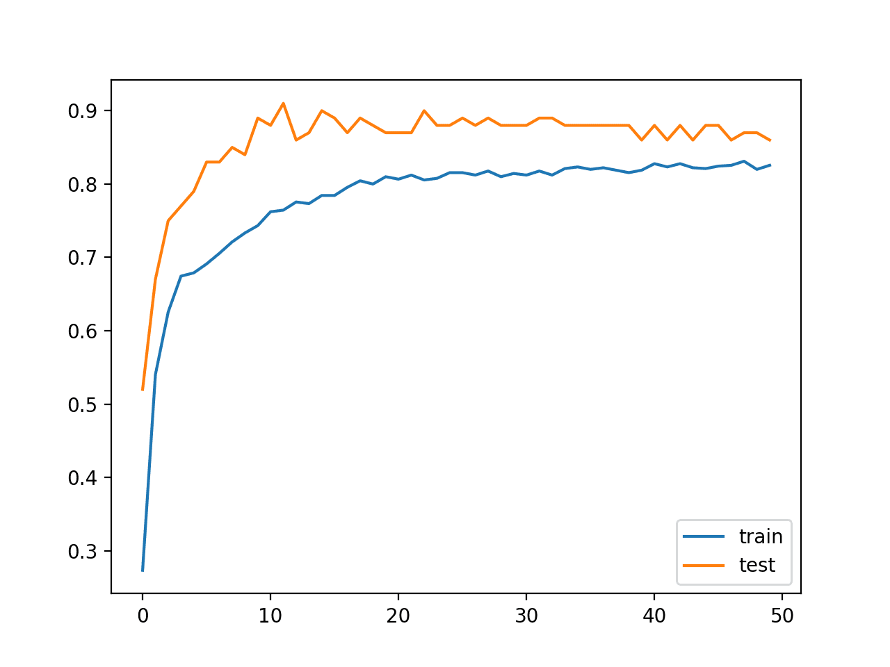
Line Plot Learning Curves of Model Accuracy on Train and Test Dataset Over Each Training Epoch
Random Splits Ensemble
The instability of the model and the small test dataset mean that we don’t really know how well this model will perform on new data in general.
We can try a simple resampling method of repeatedly generating new random splits of the dataset in train and test sets and fit new models. Calculating the average of the performance of the model across each split will give a better estimate of the model’s generalization error.
We can then combine multiple models trained on the random splits with the expectation that performance of the ensemble is likely to be more stable and better than the average single model.
We will generate 10 times more sample points from the problem domain and hold them back as an unseen dataset. The evaluation of a model on this much larger dataset will be used as a proxy or a much more accurate estimate of the generalization error of a model for this problem.
This extra dataset is not a test dataset. Technically, it is for the purposes of this demonstration, but we are pretending that this data is unavailable at model training time.
# generate 2d classification dataset
dataX, datay = make_blobs(n_samples=55000, centers=3, n_features=2, cluster_std=2, random_state=2)
X, newX = dataX[:5000, :], dataX[5000:, :]
y, newy = datay[:5000], datay[5000:]
So now we have 5,000 examples to train our model and estimate its general performance. We also have 50,000 examples that we can use to better approximate the true general performance of a single model or an ensemble.
Next, we need a function to fit and evaluate a single model on a training dataset and return the performance of the fit model on a test dataset. We also need the model that was fit so that we can use it as part of an ensemble. The evaluate_model() function below implements this behavior.
# evaluate a single mlp model
def evaluate_model(trainX, trainy, testX, testy):
	# encode targets
	trainy_enc = to_categorical(trainy)
	testy_enc = to_categorical(testy)
	# define model
	model = Sequential()
	model.add(Dense(50, input_dim=2, activation='relu'))
	model.add(Dense(3, activation='softmax'))
	model.compile(loss='categorical_crossentropy', optimizer='adam', metrics=['accuracy'])
	# fit model
	model.fit(trainX, trainy_enc, epochs=50, verbose=0)
	# evaluate the model
	_, test_acc = model.evaluate(testX, testy_enc, verbose=0)
	return model, test_acc
Next, we can create random splits of the training dataset and fit and evaluate models on each split.
We can use the train_test_split() function from the scikit-learn library to create a random split of a dataset into train and test sets. It takes the X and y arrays as arguments and the “test_size” specifies the size of the test dataset in terms of a percentage. We will use 10% of the 5,000 examples as the test.
We can then call the evaluate_model() to fit and evaluate a model. The returned accuracy and model can then be added to lists for later use.
In this example, we will limit the number of splits, and in turn, the number of fit models to 10.
# multiple train-test splits
n_splits = 10
scores, members = list(), list()
for _ in range(n_splits):
	# split data
	trainX, testX, trainy, testy = train_test_split(X, y, test_size=0.10)
	# evaluate model
	model, test_acc = evaluate_model(trainX, trainy, testX, testy)
	print('>%.3f' % test_acc)
	scores.append(test_acc)
	members.append(model)
After fitting and evaluating the models, we can estimate the expected performance of a given model with the chosen configuration for the domain.
# summarize expected performance
print('Estimated Accuracy %.3f (%.3f)' % (mean(scores), std(scores)))
We don’t know how many of the models will be useful in the ensemble. It is likely that there will be a point of diminishing returns, after which the addition of further members no longer changes the performance of the ensemble.
Nevertheless, we can evaluate different ensemble sizes from 1 to 10 and plot their performance on the unseen holdout dataset.
We can also evaluate each model on the holdout dataset and calculate the average of these scores to get a much better approximation of the true performance of the chosen model on the prediction problem.
# evaluate different numbers of ensembles on hold out set
single_scores, ensemble_scores = list(), list()
for i in range(1, n_splits+1):
	ensemble_score = evaluate_n_members(members, i, newX, newy)
	newy_enc = to_categorical(newy)
	_, single_score = members[i-1].evaluate(newX, newy_enc, verbose=0)
	print('> %d: single=%.3f, ensemble=%.3f' % (i, single_score, ensemble_score))
	ensemble_scores.append(ensemble_score)
	single_scores.append(single_score)
Finally, we can compare and calculate a more robust estimate of the general performance of an average model on the prediction problem, then plot the performance of the ensemble size to accuracy on the holdout dataset.
# plot score vs number of ensemble members
print('Accuracy %.3f (%.3f)' % (mean(single_scores), std(single_scores)))
x_axis = [i for i in range(1, n_splits+1)]
pyplot.plot(x_axis, single_scores, marker='o', linestyle='None')
pyplot.plot(x_axis, ensemble_scores, marker='o')
pyplot.show()
Tying all of this together, the complete example is listed below.
# random-splits mlp ensemble on blobs dataset
from sklearn.datasets.samples_generator import make_blobs
from sklearn.model_selection import train_test_split
from sklearn.metrics import accuracy_score
from keras.utils import to_categorical
from keras.models import Sequential
from keras.layers import Dense
from matplotlib import pyplot
from numpy import mean
from numpy import std
import numpy
from numpy import array
from numpy import argmax

# evaluate a single mlp model
def evaluate_model(trainX, trainy, testX, testy):
	# encode targets
	trainy_enc = to_categorical(trainy)
	testy_enc = to_categorical(testy)
	# define model
	model = Sequential()
	model.add(Dense(50, input_dim=2, activation='relu'))
	model.add(Dense(3, activation='softmax'))
	model.compile(loss='categorical_crossentropy', optimizer='adam', metrics=['accuracy'])
	# fit model
	model.fit(trainX, trainy_enc, epochs=50, verbose=0)
	# evaluate the model
	_, test_acc = model.evaluate(testX, testy_enc, verbose=0)
	return model, test_acc

# make an ensemble prediction for multi-class classification
def ensemble_predictions(members, testX):
	# make predictions
	yhats = [model.predict(testX) for model in members]
	yhats = array(yhats)
	# sum across ensemble members
	summed = numpy.sum(yhats, axis=0)
	# argmax across classes
	result = argmax(summed, axis=1)
	return result

# evaluate a specific number of members in an ensemble
def evaluate_n_members(members, n_members, testX, testy):
	# select a subset of members
	subset = members[:n_members]
	# make prediction
	yhat = ensemble_predictions(subset, testX)
	# calculate accuracy
	return accuracy_score(testy, yhat)

# generate 2d classification dataset
dataX, datay = make_blobs(n_samples=55000, centers=3, n_features=2, cluster_std=2, random_state=2)
X, newX = dataX[:5000, :], dataX[5000:, :]
y, newy = datay[:5000], datay[5000:]
# multiple train-test splits
n_splits = 10
scores, members = list(), list()
for _ in range(n_splits):
	# split data
	trainX, testX, trainy, testy = train_test_split(X, y, test_size=0.10)
	# evaluate model
	model, test_acc = evaluate_model(trainX, trainy, testX, testy)
	print('>%.3f' % test_acc)
	scores.append(test_acc)
	members.append(model)
# summarize expected performance
print('Estimated Accuracy %.3f (%.3f)' % (mean(scores), std(scores)))
# evaluate different numbers of ensembles on hold out set
single_scores, ensemble_scores = list(), list()
for i in range(1, n_splits+1):
	ensemble_score = evaluate_n_members(members, i, newX, newy)
	newy_enc = to_categorical(newy)
	_, single_score = members[i-1].evaluate(newX, newy_enc, verbose=0)
	print('> %d: single=%.3f, ensemble=%.3f' % (i, single_score, ensemble_score))
	ensemble_scores.append(ensemble_score)
	single_scores.append(single_score)
# plot score vs number of ensemble members
print('Accuracy %.3f (%.3f)' % (mean(single_scores), std(single_scores)))
x_axis = [i for i in range(1, n_splits+1)]
pyplot.plot(x_axis, single_scores, marker='o', linestyle='None')
pyplot.plot(x_axis, ensemble_scores, marker='o')
pyplot.show()
Running the example first fits and evaluates 10 models on 10 different random splits of the dataset into train and test sets.
From these scores, we estimate that the average model fit on the dataset will achieve an accuracy of about 83% with a standard deviation of about 1.9%.
>0.816
>0.836
>0.818
>0.806
>0.814
>0.824
>0.830
>0.848
>0.868
>0.858
Estimated Accuracy 0.832 (0.019)
We then evaluate the performance of each model on the unseen dataset and the performance of ensembles of models from 1 to 10 models.
From these scores, we can see that a more accurate estimate of the performance of an average model on this problem is about 82% and that the estimated performance is optimistic.
> 1: single=0.821, ensemble=0.821
> 2: single=0.821, ensemble=0.820
> 3: single=0.820, ensemble=0.820
> 4: single=0.820, ensemble=0.821
> 5: single=0.821, ensemble=0.821
> 6: single=0.820, ensemble=0.821
> 7: single=0.820, ensemble=0.821
> 8: single=0.820, ensemble=0.821
> 9: single=0.820, ensemble=0.820
> 10: single=0.820, ensemble=0.821
Accuracy 0.820 (0.000)
A lot of the difference between the accuracy scores is happening in the fractions of percent.
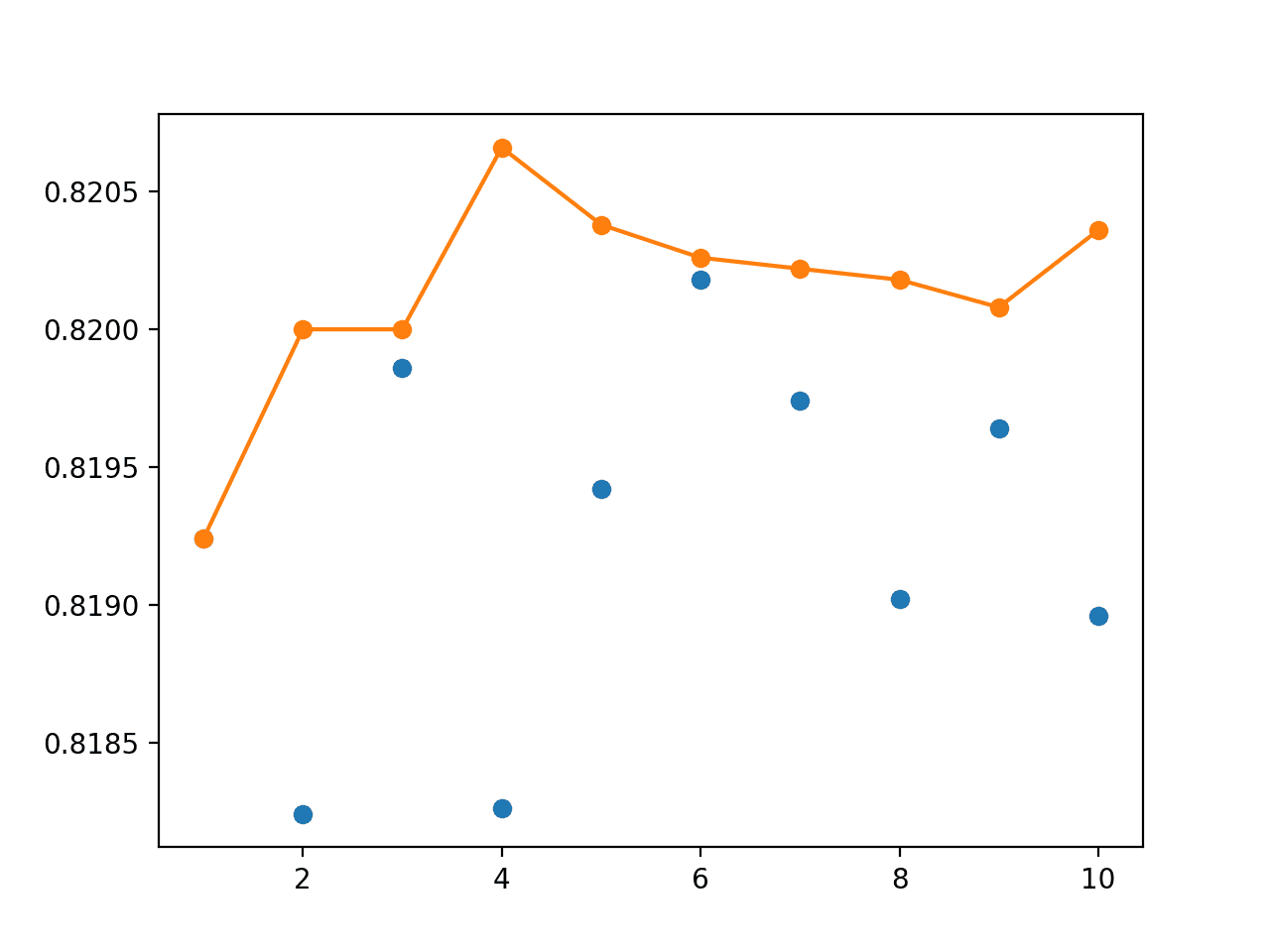
A graph is created showing the accuracy of each individual model on the unseen holdout dataset as blue dots and the performance of an ensemble with a given number of members from 1-10 as an orange line and dots.
We can see that using an ensemble of 4-to-8 members, at least in this case, results in an accuracy that is better than most of the individual runs (orange line is above many blue dots).
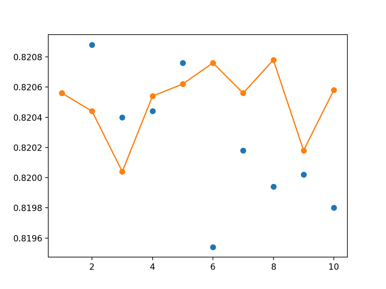
Line Plot Showing Single Model Accuracy (blue dots) vs Accuracy of Ensembles of Varying Size for Random-Split Resampling
The graph does show some individual models can perform better than an ensemble of models (blue dots above the orange line), but we are unable to choose these models. Here, we demonstrate that without additional data (e.g. the out of sample dataset) that an ensemble of 4-to-8 members will give better on average performance than a randomly selected train-test model.
More repeats (e.g. 30 or 100) may result in a more stable ensemble performance.
Cross-Validation Ensemble
A problem with repeated random splits as a resampling method for estimating the average performance of model is that it is optimistic.
An approach designed to be less optimistic and is widely used as a result is the k-fold cross-validation method.
The method is less biased because each example in the dataset is only used one time in the test dataset to estimate model performance, unlike random train-test splits where a given example may be used to evaluate a model many times.
The procedure has a single parameter called k that refers to the number of groups that a given data sample is to be split into. The average of the scores of each model provides a less biased estimate of model performance. A typical value for k is 10.
Because neural network models are computationally very expensive to train, it is common to use the best performing model during cross-validation as the final model.
Alternately, the resulting models from the cross-validation process can be combined to provide a cross-validation ensemble that is likely to have better performance on average than a given single model.
We can use the KFold class from scikit-learn to split the dataset into k folds. It takes as arguments the number of splits, whether or not to shuffle the sample, and the seed for the pseudorandom number generator used prior to the shuffle.
# prepare the k-fold cross-validation configuration
n_folds = 10
kfold = KFold(n_folds, True, 1)
Once the class is instantiated, it can be enumerated to get each split of indexes into the dataset for the train and test sets.
# cross validation estimation of performance
scores, members = list(), list()
for train_ix, test_ix in kfold.split(X):
	# select samples
	trainX, trainy = X[train_ix], y[train_ix]
	testX, testy = X[test_ix], y[test_ix]
	# evaluate model
	model, test_acc = evaluate_model(trainX, trainy, testX, testy)
	print('>%.3f' % test_acc)
	scores.append(test_acc)
	members.append(model)
Once the scores are calculated on each fold, the average of the scores can be used to report the expected performance of the approach.
# summarize expected performance
print('Estimated Accuracy %.3f (%.3f)' % (mean(scores), std(scores)))
Now that we have collected the 10 models evaluated on the 10 folds, we can use them to create a cross-validation ensemble. It seems intuitive to use all 10 models in the ensemble, nevertheless, we can evaluate the accuracy of each subset of ensembles from 1 to 10 members as we did in the previous section.
The complete example of analyzing the cross-validation ensemble is listed below.
# cross-validation mlp ensemble on blobs dataset
from sklearn.datasets.samples_generator import make_blobs
from sklearn.model_selection import KFold
from sklearn.metrics import accuracy_score
from keras.utils import to_categorical
from keras.models import Sequential
from keras.layers import Dense
from matplotlib import pyplot
from numpy import mean
from numpy import std
import numpy
from numpy import array
from numpy import argmax

# evaluate a single mlp model
def evaluate_model(trainX, trainy, testX, testy):
	# encode targets
	trainy_enc = to_categorical(trainy)
	testy_enc = to_categorical(testy)
	# define model
	model = Sequential()
	model.add(Dense(50, input_dim=2, activation='relu'))
	model.add(Dense(3, activation='softmax'))
	model.compile(loss='categorical_crossentropy', optimizer='adam', metrics=['accuracy'])
	# fit model
	model.fit(trainX, trainy_enc, epochs=50, verbose=0)
	# evaluate the model
	_, test_acc = model.evaluate(testX, testy_enc, verbose=0)
	return model, test_acc

# make an ensemble prediction for multi-class classification
def ensemble_predictions(members, testX):
	# make predictions
	yhats = [model.predict(testX) for model in members]
	yhats = array(yhats)
	# sum across ensemble members
	summed = numpy.sum(yhats, axis=0)
	# argmax across classes
	result = argmax(summed, axis=1)
	return result

# evaluate a specific number of members in an ensemble
def evaluate_n_members(members, n_members, testX, testy):
	# select a subset of members
	subset = members[:n_members]
	# make prediction
	yhat = ensemble_predictions(subset, testX)
	# calculate accuracy
	return accuracy_score(testy, yhat)

# generate 2d classification dataset
dataX, datay = make_blobs(n_samples=55000, centers=3, n_features=2, cluster_std=2, random_state=2)
X, newX = dataX[:5000, :], dataX[5000:, :]
y, newy = datay[:5000], datay[5000:]
# prepare the k-fold cross-validation configuration
n_folds = 10
kfold = KFold(n_folds, True, 1)
# cross validation estimation of performance
scores, members = list(), list()
for train_ix, test_ix in kfold.split(X):
	# select samples
	trainX, trainy = X[train_ix], y[train_ix]
	testX, testy = X[test_ix], y[test_ix]
	# evaluate model
	model, test_acc = evaluate_model(trainX, trainy, testX, testy)
	print('>%.3f' % test_acc)
	scores.append(test_acc)
	members.append(model)
# summarize expected performance
print('Estimated Accuracy %.3f (%.3f)' % (mean(scores), std(scores)))
# evaluate different numbers of ensembles on hold out set
single_scores, ensemble_scores = list(), list()
for i in range(1, n_folds+1):
	ensemble_score = evaluate_n_members(members, i, newX, newy)
	newy_enc = to_categorical(newy)
	_, single_score = members[i-1].evaluate(newX, newy_enc, verbose=0)
	print('> %d: single=%.3f, ensemble=%.3f' % (i, single_score, ensemble_score))
	ensemble_scores.append(ensemble_score)
	single_scores.append(single_score)
# plot score vs number of ensemble members
print('Accuracy %.3f (%.3f)' % (mean(single_scores), std(single_scores)))
x_axis = [i for i in range(1, n_folds+1)]
pyplot.plot(x_axis, single_scores, marker='o', linestyle='None')
pyplot.plot(x_axis, ensemble_scores, marker='o')
pyplot.show()
Running the example first prints the performance of each of the 10 models on each of the folds of the cross-validation.
The average performance of these models is reported as about 82%, which appears to be less optimistic than the random-splits approach used in the previous section.
>0.834
>0.870
>0.818
>0.806
>0.836
>0.804
>0.820
>0.830
>0.828
>0.822
Estimated Accuracy 0.827 (0.018)
Next, each of the saved models is evaluated on the unseen holdout set.
The average of these scores is also about 82%, highlighting that, at least in this case, the cross-validation estimation of the general performance of the model was reasonable.
> 1: single=0.819, ensemble=0.819
> 2: single=0.820, ensemble=0.820
> 3: single=0.820, ensemble=0.820
> 4: single=0.821, ensemble=0.821
> 5: single=0.820, ensemble=0.821
> 6: single=0.821, ensemble=0.821
> 7: single=0.820, ensemble=0.820
> 8: single=0.819, ensemble=0.821
> 9: single=0.820, ensemble=0.821
> 10: single=0.820, ensemble=0.821
Accuracy 0.820 (0.001)
A graph of single model accuracy (blue dots) and ensemble size vs accuracy (orange line) is created.
As in the previous example, the real difference between the performance of the models is in the fractions of percent in model accuracy.
The orange line shows that as the number of members increases, the accuracy of the ensemble increases to a point of diminishing returns.
We can see that, at least in this case, using four or more of the models fit during cross-validation in an ensemble gives better performance than almost all individual models.
We can also see that a default strategy of using all models in the ensemble would be effective.
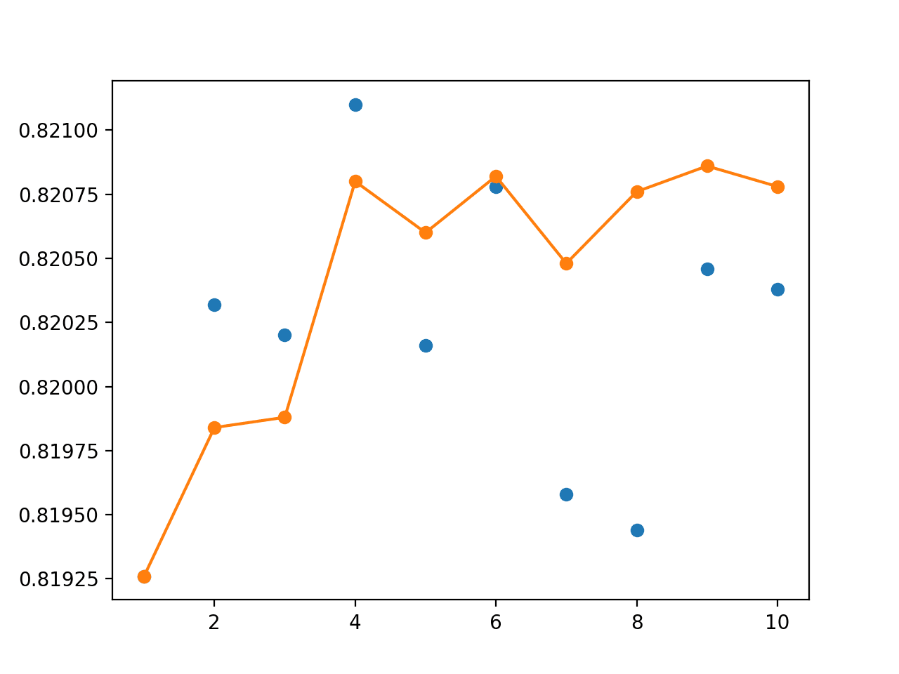
Line Plot Showing Single Model Accuracy (blue dots) vs Accuracy of Ensembles of Varying Size for Cross-Validation Resampling
Bagging Ensemble
A limitation of random splits and k-fold cross-validation from the perspective of ensemble learning is that the models are very similar.
The bootstrap method is a statistical technique for estimating quantities about a population by averaging estimates from multiple small data samples.
Importantly, samples are constructed by drawing observations from a large data sample one at a time and returning them to the data sample after they have been chosen. This allows a given observation to be included in a given small sample more than once. This approach to sampling is called sampling with replacement.
The method can be used to estimate the performance of neural network models. Examples not selected in a given sample can be used as a test set to estimate the performance of the model.
The bootstrap is a robust method for estimating model performance. It does suffer a little from an optimistic bias, but is often almost as accurate as k-fold cross-validation in practice.
The benefit for ensemble learning is that each model is that each data sample is biased, allowing a given example to appear many times in the sample. This, in turn, means that the models trained on those samples will be biased, importantly in different ways. The result can be ensemble predictions that can be more accurate.
Generally, use of the bootstrap method in ensemble learning is referred to as bootstrap aggregation or bagging.
We can use the resample() function from scikit-learn to select a subsample with replacement. The function takes an array to subsample and the size of the resample as arguments. We will perform the selection in rows indices that we can in turn use to select rows in the X and y arrays.
The size of the sample will be 4,500, or 90% of the data, although the test set may be larger than 10% as given the use of resampling, more than 500 examples may have been left unselected.
# multiple train-test splits
n_splits = 10
scores, members = list(), list()
for _ in range(n_splits):
	# select indexes
	ix = [i for i in range(len(X))]
	train_ix = resample(ix, replace=True, n_samples=4500)
	test_ix = [x for x in ix if x not in train_ix]
	# select data
	trainX, trainy = X[train_ix], y[train_ix]
	testX, testy = X[test_ix], y[test_ix]
	# evaluate model
	model, test_acc = evaluate_model(trainX, trainy, testX, testy)
	print('>%.3f' % test_acc)
	scores.append(test_acc)
	members.append(model)
It is common to use simple overfit models like unpruned decision trees when using a bagging ensemble learning strategy.
Better performance may be seen with over-constrained and overfit neural networks. Nevertheless, we will use the same MLP from previous sections in this example.
Additionally, it is common to continue to add ensemble members in bagging until the performance of the ensemble plateaus, as bagging does not overfit the dataset. We will again limit the number of members to 10 as in previous examples.
The complete example of bootstrap aggregation for estimating model performance and ensemble learning with a Multilayer Perceptron is listed below.
# bagging mlp ensemble on blobs dataset
from sklearn.datasets.samples_generator import make_blobs
from sklearn.utils import resample
from sklearn.metrics import accuracy_score
from keras.utils import to_categorical
from keras.models import Sequential
from keras.layers import Dense
from matplotlib import pyplot
from numpy import mean
from numpy import std
import numpy
from numpy import array
from numpy import argmax

# evaluate a single mlp model
def evaluate_model(trainX, trainy, testX, testy):
	# encode targets
	trainy_enc = to_categorical(trainy)
	testy_enc = to_categorical(testy)
	# define model
	model = Sequential()
	model.add(Dense(50, input_dim=2, activation='relu'))
	model.add(Dense(3, activation='softmax'))
	model.compile(loss='categorical_crossentropy', optimizer='adam', metrics=['accuracy'])
	# fit model
	model.fit(trainX, trainy_enc, epochs=50, verbose=0)
	# evaluate the model
	_, test_acc = model.evaluate(testX, testy_enc, verbose=0)
	return model, test_acc

# make an ensemble prediction for multi-class classification
def ensemble_predictions(members, testX):
	# make predictions
	yhats = [model.predict(testX) for model in members]
	yhats = array(yhats)
	# sum across ensemble members
	summed = numpy.sum(yhats, axis=0)
	# argmax across classes
	result = argmax(summed, axis=1)
	return result

# evaluate a specific number of members in an ensemble
def evaluate_n_members(members, n_members, testX, testy):
	# select a subset of members
	subset = members[:n_members]
	# make prediction
	yhat = ensemble_predictions(subset, testX)
	# calculate accuracy
	return accuracy_score(testy, yhat)

# generate 2d classification dataset
dataX, datay = make_blobs(n_samples=55000, centers=3, n_features=2, cluster_std=2, random_state=2)
X, newX = dataX[:5000, :], dataX[5000:, :]
y, newy = datay[:5000], datay[5000:]
# multiple train-test splits
n_splits = 10
scores, members = list(), list()
for _ in range(n_splits):
	# select indexes
	ix = [i for i in range(len(X))]
	train_ix = resample(ix, replace=True, n_samples=4500)
	test_ix = [x for x in ix if x not in train_ix]
	# select data
	trainX, trainy = X[train_ix], y[train_ix]
	testX, testy = X[test_ix], y[test_ix]
	# evaluate model
	model, test_acc = evaluate_model(trainX, trainy, testX, testy)
	print('>%.3f' % test_acc)
	scores.append(test_acc)
	members.append(model)
# summarize expected performance
print('Estimated Accuracy %.3f (%.3f)' % (mean(scores), std(scores)))
# evaluate different numbers of ensembles on hold out set
single_scores, ensemble_scores = list(), list()
for i in range(1, n_splits+1):
	ensemble_score = evaluate_n_members(members, i, newX, newy)
	newy_enc = to_categorical(newy)
	_, single_score = members[i-1].evaluate(newX, newy_enc, verbose=0)
	print('> %d: single=%.3f, ensemble=%.3f' % (i, single_score, ensemble_score))
	ensemble_scores.append(ensemble_score)
	single_scores.append(single_score)
# plot score vs number of ensemble members
print('Accuracy %.3f (%.3f)' % (mean(single_scores), std(single_scores)))
x_axis = [i for i in range(1, n_splits+1)]
pyplot.plot(x_axis, single_scores, marker='o', linestyle='None')
pyplot.plot(x_axis, ensemble_scores, marker='o')
pyplot.show()
Running the example prints the model performance on the unused examples for each bootstrap sample.
We can see that, in this case, the expected performance of the model is less optimistic than random train-test splits and is perhaps quite similar to the finding for k-fold cross-validation.
>0.829
>0.820
>0.830
>0.821
>0.831
>0.820
>0.834
>0.815
>0.829
>0.827
Estimated Accuracy 0.825 (0.006)
Perhaps due to the bootstrap sampling procedure, we see that the actual performance of each model is a little worse on the much larger unseen holdout dataset.
This is to be expected given the bias introduced by the sampling with replacement of the bootstrap.
> 1: single=0.819, ensemble=0.819
> 2: single=0.818, ensemble=0.820
> 3: single=0.820, ensemble=0.820
> 4: single=0.818, ensemble=0.821
> 5: single=0.819, ensemble=0.820
> 6: single=0.820, ensemble=0.820
> 7: single=0.820, ensemble=0.820
> 8: single=0.819, ensemble=0.820
> 9: single=0.820, ensemble=0.820
> 10: single=0.819, ensemble=0.820
Accuracy 0.819 (0.001)
The created line plot is encouraging.
We see that after about four members that the bagged ensemble achieves better performance on the holdout dataset than any individual model. No doubt, given the slightly lower average performance of individual models.
Line Plot Showing Single Model Accuracy (blue dots) vs Accuracy of Ensembles of Varying Size for Bagging
Extensions
This section lists some ideas for extending the tutorial that you may wish to explore.
- Single Model. Compare the performance of each ensemble to one model trained on all available data.
- CV Ensemble Size. Experiment with larger and smaller ensemble sizes for the cross-validation ensemble and compare their performance.
- Bagging Ensemble Limit. Increase the number of members in the bagging ensemble to find the point of diminishing returns.
If you explore any of these extensions, I’d love to know.
Further Reading
This section provides more resources on the topic if you are looking to go deeper.
Posts
- A Gentle Introduction to k-fold Cross-Validation
- A Gentle Introduction to the Bootstrap Method
- How to Implement Bagging From Scratch With Python
Papers
API
- Getting started with the Keras Sequential model
- Keras Core Layers API
- scipy.stats.mode API
- numpy.argmax API
- sklearn.datasets.make_blobs API
- sklearn.model_selection.train_test_split API
- sklearn.model_selection.KFold API
- sklearn.utils.resample API
Summary
In this tutorial, you discovered how to develop a suite of different resampling-based ensembles for deep learning neural network models.
Specifically, you learned:
- How to estimate model performance using random-splits and develop an ensemble from the models.
- How to estimate performance using 10-fold cross-validation and develop a cross-validation ensemble.
- How to estimate performance using the bootstrap and combine models using a bagging ensemble.
Do you have any questions?
Ask your questions in the comments below and I will do my best to answer.
The post How to Create a Random-Split, Cross-Validation, and Bagging Ensemble for Deep Learning in Keras appeared first on Machine Learning Mastery.