
Author: Jason Brownlee
Predictive modeling problems where the training dataset is small relative to the number of unlabeled examples are challenging.
Neural networks can perform well on these types of problems, although they can suffer from high variance in model performance as measured on a training or hold-out validation datasets. This makes choosing which model to use as the final model risky, as there is no clear signal as to which model is better than another toward the end of the training run.
The horizontal voting ensemble is a simple method to address this issue, where a collection of models saved over contiguous training epochs towards the end of a training run are saved and used as an ensemble that results in more stable and better performance on average than randomly choosing a single final model.
In this tutorial, you will discover how to reduce the variance of a final deep learning neural network model using a horizontal voting ensemble.
After completing this tutorial, you will know:
- That it is challenging to choose a final neural network model that has high variance on a training dataset.
- Horizontal voting ensembles provide a way to reduce variance and improve average model performance for models with high variance using a single training run.
- How to develop a horizontal voting ensemble in Python using Keras to improve the performance of a final multilayer Perceptron model for multi-class classification.
Let’s get started.

How to Reduce Variance in the Final Deep Learning Model With a Horizontal Voting Ensemble
Photo by Fatima Flores, some rights reserved.
Tutorial Overview
This tutorial is divided into five parts; they are:
- Horizontal Voting Ensemble
- Multi-Class Classification Problem
- Multilayer Perceptron Model
- Save Horizontal Models
- Make Horizontal Ensemble Predictions
Horizontal Voting Ensemble
Ensemble learning combines the predictions from multiple models.
A challenge when using ensemble learning when using deep learning methods is that given the use of very large datasets and large models, a given training run may take days, weeks, or even months. Training multiple models may not be feasible.
An alternative source of models that may contribute to an ensemble are the state of a single model at different points during training.
Horizontal voting is an ensemble method proposed by Jingjing Xie, et al. in their 2013 paper “Horizontal and Vertical Ensemble with Deep Representation for Classification.”
The method involves using multiple models from the end of a contiguous block of epochs before the end of training in an ensemble to make predictions.
The approach was developed specifically for those predictive modeling problems where the training dataset is relatively small compared to the number of predictions required by the model. This results in a model that has a high variance in performance during training. In this situation, using the final model or any given model toward the end of the training process is risky given the variance in performance.
… the error rate of classification would first decline and then tend to be stable with the training epoch grows. But when size of labeled training set is too small, the error rate would oscillate […] So it is difficult to choose a “magic” epoch to obtain a reliable output.
— Horizontal and Vertical Ensemble with Deep Representation for Classification, 2013.
Instead, the authors suggest using all of the models in an ensemble from a contiguous block of epochs during training, such as models from the last 200 epochs. The result are predictions by the ensemble that are as good as or better than any single model in the ensemble.
To reduce the instability, we put forward a method called Horizontal Voting. First, networks trained for a relatively stable range of epoch are selected. The predictions of the probability of each label are produced by standard classifiers with top level representation of the selected epoch, and then averaged.
— Horizontal and Vertical Ensemble with Deep Representation for Classification, 2013.
As such, the horizontal voting ensemble method provides an ideal method for both cases where a given model requires vast computational resources to train, and/or cases where final model selection is challenging given the high variance of training due to the use of a relatively small training dataset.
Now that are we are familiar with horizontal voting, we can implement the procedure.
Want Better Results with Deep Learning?
Take my free 7-day email crash course now (with sample code).
Click to sign-up and also get a free PDF Ebook version of the course.
Multi-Class Classification Problem
We will use a small multi-class classification problem as the basis to demonstrate a horizontal voting ensemble.
The scikit-learn class provides the make_blobs() function that can be used to create a multi-class classification problem with the prescribed number of samples, input variables, classes, and variance of samples within a class.
The problem has two input variables (to represent the x and y coordinates of the points) and a standard deviation of 2.0 for points within each group. We will use the same random state (seed for the pseudorandom number generator) to ensure that we always get the same data points.
# generate 2d classification dataset
X, y = make_blobs(n_samples=1000, centers=3, n_features=2, cluster_std=2, random_state=2)
The results are the input and output elements of a dataset that we can model.
In order to get a feeling for the complexity of the problem, we can graph each point on a two-dimensional scatter plot and color each point by class value.
The complete example is listed below.
# scatter plot of blobs dataset
from sklearn.datasets.samples_generator import make_blobs
from matplotlib import pyplot
from pandas import DataFrame
# generate 2d classification dataset
X, y = make_blobs(n_samples=1000, centers=3, n_features=2, cluster_std=2, random_state=2)
# scatter plot, dots colored by class value
df = DataFrame(dict(x=X[:,0], y=X[:,1], label=y))
colors = {0:'red', 1:'blue', 2:'green'}
fig, ax = pyplot.subplots()
grouped = df.groupby('label')
for key, group in grouped:
    group.plot(ax=ax, kind='scatter', x='x', y='y', label=key, color=colors[key])
pyplot.show()
Running the example creates a scatter plot of the entire dataset. We can see that the standard deviation of 2.0 means that the classes are not linearly separable (can be separated by a line) causing many ambiguous points.
This is desirable as it means that the problem is non-trivial and will allow a neural network model to find many different “good enough” candidate solutions resulting in a high variance.
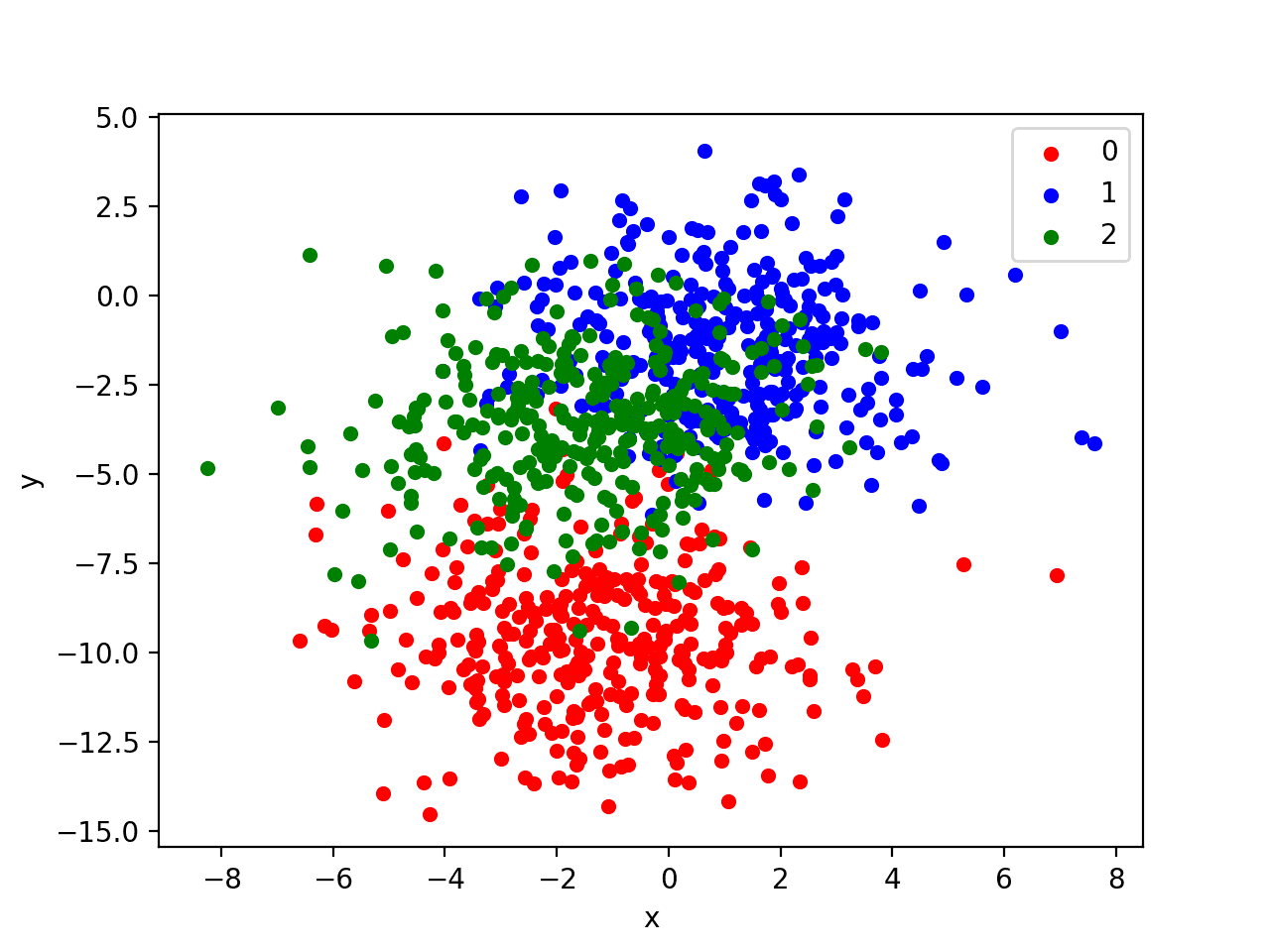
Scatter Plot of Blobs Dataset With Three Classes and Points Colored by Class Value
Multilayer Perceptron Model
Before we define a model, we need to contrive a problem that is appropriate for a horizontal voting ensemble.
In our problem, the training dataset is relatively small. Specifically, there is a 10:1 ratio of examples in the training dataset to the holdout dataset. This mimics a situation where we may have a vast number of unlabeled examples and a small number of labeled examples with which to train a model.
We will create 1,100 data points from the blobs problem. The model will be trained on the first 100 points and the remaining 1,000 will be held back in a test dataset, unavailable to the model.
# generate 2d classification dataset
X, y = make_blobs(n_samples=1100, centers=3, n_features=2, cluster_std=2, random_state=2)
# split into train and test
n_train = 100
trainX, testX = X[:n_train, :], X[n_train:, :]
trainy, testy = y[:n_train], y[n_train:]
print(trainX.shape, testX.shape)
The problem is a multi-class classification problem, and we will model it using a softmax activation function on the output layer.
This means that the model will predict a vector with three elements with the probability that the sample belongs to each of the three classes. Therefore, we must one hot encode the class values, ideally before we split the rows into the train, test, and validation datasets so that it is a single function call.
y = to_categorical(y)
Next, we can define and combine the model.
The model will expect samples with two input variables. The model then has a single hidden layer with 25 nodes and a rectified linear activation function, then an output layer with three nodes to predict the probability of each of the three classes and a softmax activation function.
Because the problem is multi-class, we will use the categorical cross entropy loss function to optimize the model and the efficient Adam flavor of stochastic gradient descent.
# define model
model = Sequential()
model.add(Dense(25, input_dim=2, activation='relu'))
model.add(Dense(3, activation='softmax'))
model.compile(loss='categorical_crossentropy', optimizer='adam', metrics=['accuracy'])
The model is fit for 1,000 training epochs and we will evaluate the model each epoch on the training set, using the test set as a validation set.
# fit model
history = model.fit(trainX, trainy, validation_data=(valX, valy), epochs=1000, verbose=0)
At the end of the run, we will evaluate the performance of the model on the train, validation, and test sets.
# evaluate the model
_, train_acc = model.evaluate(trainX, trainy, verbose=0)
_, val_acc = model.evaluate(valX, valy, verbose=0)
_, test_acc = model.evaluate(testX, testy, verbose=0)
print('Train: %.3f, Validation: %.3f, Test: %.3f' % (train_acc, val_acc, test_acc))
Then finally, we will plot learning curves of the model accuracy over each training epoch on both the training and validation datasets.
# learning curves of model accuracy
pyplot.plot(history.history['acc'], label='train')
pyplot.plot(history.history['val_acc'], label='test')
pyplot.legend()
pyplot.show()
Tying all of this together, the complete example is listed below.
# develop an mlp for blobs dataset
from sklearn.datasets.samples_generator import make_blobs
from keras.utils import to_categorical
from keras.models import Sequential
from keras.layers import Dense
from matplotlib import pyplot
# generate 2d classification dataset
X, y = make_blobs(n_samples=1100, centers=3, n_features=2, cluster_std=2, random_state=2)
# one hot encode output variable
y = to_categorical(y)
# split into train and test
n_train = 100
trainX, testX = X[:n_train, :], X[n_train:, :]
trainy, testy = y[:n_train], y[n_train:]
print(trainX.shape, testX.shape)
# define model
model = Sequential()
model.add(Dense(25, input_dim=2, activation='relu'))
model.add(Dense(3, activation='softmax'))
model.compile(loss='categorical_crossentropy', optimizer='adam', metrics=['accuracy'])
# fit model
history = model.fit(trainX, trainy, validation_data=(testX, testy), epochs=1000, verbose=0)
# evaluate the model
_, train_acc = model.evaluate(trainX, trainy, verbose=0)
_, test_acc = model.evaluate(testX, testy, verbose=0)
print('Train: %.3f, Test: %.3f' % (train_acc, test_acc))
# learning curves of model accuracy
pyplot.plot(history.history['acc'], label='train')
pyplot.plot(history.history['val_acc'], label='test')
pyplot.legend()
pyplot.show()
Running the example first prints the shape of each dataset for confirmation, then the performance of the final model on the train and test datasets.
Your specific results will vary (by design!) given the high variance nature of the model.
In this case, we can see that the model achieved about 85% accuracy on the training dataset that we know is optimistic, and about 80% on the test dataset, which we would expect to be more realistic.
(100, 2) (1000, 2)
Train: 0.850, Test: 0.804
A line plot is also created showing the learning curves for the model accuracy on the train and test sets over each training epoch.
We can see that training accuracy is more optimistic over the whole run as we also noted with the final scores. We can see that the accuracy of the model has high variance on the training dataset as compared to the test set, as we would expect.
The variance in the model highlights the fact that choosing the model at the end of the run or any model from about epoch 800 is challenging as accuracy on the training dataset has a high variance. We also see a muted version of the variance on the test dataset.
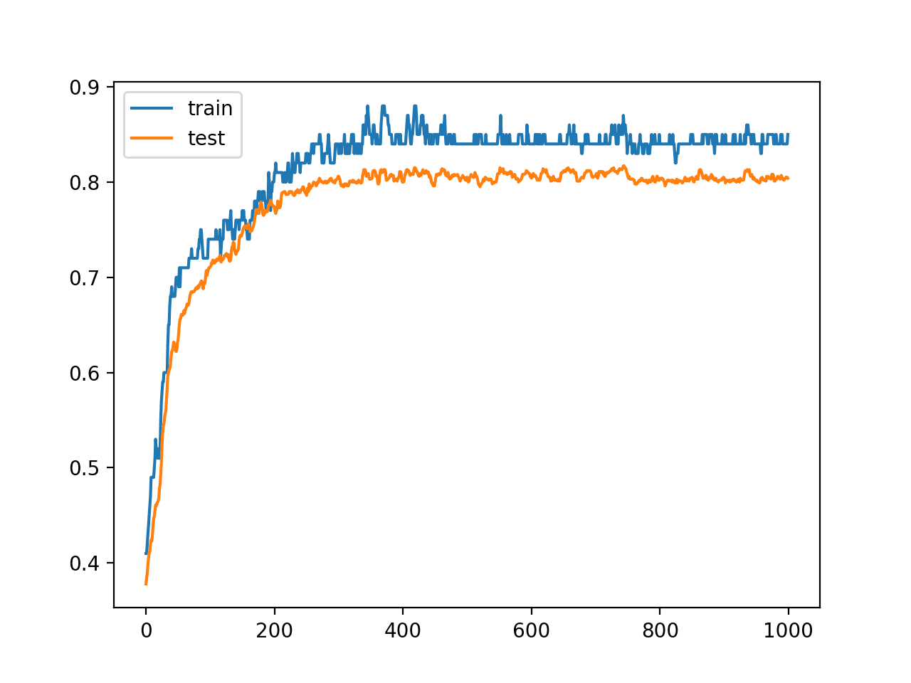
Line Plot Learning Curves of Model Accuracy on Train and Test Dataset over Each Training Epoch
Now that we have identified that the model is a good candidate for a horizontal voting ensemble, we can begin to implement the technique.
Save Horizontal Models
There may be many ways to implement a horizontal voting ensemble.
Perhaps the simplest is to manually drive the training process, one epoch at a time, then save models at the end of the epoch if we have exceeded an upper limit on the number of epochs.
For example, with our test problem, we will train the model for 1,000 epochs and perhaps save models from epoch 950 onwards (e.g. between and including epochs 950 and 999).
# fit model
n_epochs, n_save_after = 1000, 950
for i in range(n_epochs):
	# fit model for a single epoch
	model.fit(trainX, trainy, epochs=1, verbose=0)
	# check if we should save the model
	if i >= n_save_after:
		model.save('models/model_' + str(i) + '.h5')
Models can be saved to file using the save() function on the model and specifying a filename that includes the epoch number.
To avoid clutter with our source files, we will save all models under a new “models/” folder in the current working directory.
# create directory for models
makedirs('models')
Note, saving and loading neural network models in Keras requires that you have the h5py library installed.
You can install this library using pip as follows:
pip install h5py
Tying all of this together, the complete example of fitting the model on the training dataset and saving all models from the last 50 epochs is listed below.
# save horizontal voting ensemble members during training
from sklearn.datasets.samples_generator import make_blobs
from keras.utils import to_categorical
from keras.models import Sequential
from keras.layers import Dense
from matplotlib import pyplot
from os import makedirs
# generate 2d classification dataset
X, y = make_blobs(n_samples=1100, centers=3, n_features=2, cluster_std=2, random_state=2)
# one hot encode output variable
y = to_categorical(y)
# split into train and test
n_train = 100
trainX, testX = X[:n_train, :], X[n_train:, :]
trainy, testy = y[:n_train], y[n_train:]
print(trainX.shape, testX.shape)
# define model
model = Sequential()
model.add(Dense(25, input_dim=2, activation='relu'))
model.add(Dense(3, activation='softmax'))
model.compile(loss='categorical_crossentropy', optimizer='adam', metrics=['accuracy'])
# create directory for models
makedirs('models')
# fit model
n_epochs, n_save_after = 1000, 950
for i in range(n_epochs):
	# fit model for a single epoch
	model.fit(trainX, trainy, epochs=1, verbose=0)
	# check if we should save the model
	if i >= n_save_after:
		model.save('models/model_' + str(i) + '.h5')
Running the example creates the “models/” folder and saves 50 models into the directory.
Note, to re-run this example, you must delete the “models/” directory so that the script can recreate it.
Make Horizontal Ensemble Predictions
Now that we have created the models, we can use them in a horizontal voting ensemble.
First, we need to load the models into memory. This is reasonable as the models are small. If you are trying to develop a horizontal voting ensemble with very large models, it might be easier to load models one at a time, make a prediction, then load the next model and repeat the process.
The function load_all_models() below will load models from the “models/” directory. It takes the start and end epochs as arguments so that you can experiment with different groups of models saved over contiguous epochs.
# load models from file
def load_all_models(n_start, n_end):
	all_models = list()
	for epoch in range(n_start, n_end):
		# define filename for this ensemble
		filename = 'models/model_' + str(epoch) + '.h5'
		# load model from file
		model = load_model(filename)
		# add to list of members
		all_models.append(model)
		print('>loaded %s' % filename)
	return all_models
We can call the function to load all of the models.
We can then reverse the list of models so that the models at the end of the run are at the beginning of the list. This will be helpful later when we test voting ensembles of different sizes, including models sequentially from the end of the run backward through training epochs, in case the best models really were at the end of the run.
# load models in order
members = load_all_models(950, 1000)
print('Loaded %d models' % len(members))
# reverse loaded models so we build the ensemble with the last models first
members = list(reversed(members))
Next, we can evaluate each saved model on the test dataset, as well as a voting ensemble of the last n contiguous models from training.
We want to know how well each model actually performed on the test dataset and, importantly, the distribution of model performance on the test dataset, so that we know how well (or poorly) an average model chosen from the end of the run would perform in practice.
We don’t know how many members to include in the horizontal voting ensemble. Therefore, we can test different numbers of contiguous members, working backward from the final model.
First, we need a function to make a prediction with a list of ensemble members. Each member predicts the probabilities for each of the three output classes. The probabilities are added and we use an argmax to select the class with the most support. The ensemble_predictions() function below implements this voting based prediction scheme.
# make an ensemble prediction for multi-class classification
def ensemble_predictions(members, testX):
	# make predictions
	yhats = [model.predict(testX) for model in members]
	yhats = array(yhats)
	# sum across ensemble members
	summed = numpy.sum(yhats, axis=0)
	# argmax across classes
	result = argmax(summed, axis=1)
	return result
Next, we need a function to evaluate a subset of the ensemble members of a given size.
The subset needs to be selected, predictions made, and the performance of the ensemble estimated by comparing the predictions to the expected values. The evaluate_n_members() function below implements this ensemble size evaluation.
# evaluate a specific number of members in an ensemble
def evaluate_n_members(members, n_members, testX, testy):
	# select a subset of members
	subset = members[:n_members]
	# make prediction
	yhat = ensemble_predictions(subset, testX)
	# calculate accuracy
	return accuracy_score(testy, yhat)
We can now enumerate through different sized horizontal voting ensembles from 1 to 50. Each member is evaluated alone, then the ensemble of that size is evaluated and scores are recorded.
# evaluate different numbers of ensembles on hold out set
single_scores, ensemble_scores = list(), list()
for i in range(1, len(members)+1):
	# evaluate model with i members
	ensemble_score = evaluate_n_members(members, i, testX, testy)
	# evaluate the i'th model standalone
	testy_enc = to_categorical(testy)
	_, single_score = members[i-1].evaluate(testX, testy_enc, verbose=0)
	# summarize this step
	print('> %d: single=%.3f, ensemble=%.3f' % (i, single_score, ensemble_score))
	ensemble_scores.append(ensemble_score)
	single_scores.append(single_score)
At the end of the evaluations, we report the distribution of scores of single models on the test dataset. The average score is what we would expect on average if we picked any of the saved models as a final model.
# summarize average accuracy of a single final model
print('Accuracy %.3f (%.3f)' % (mean(single_scores), std(single_scores)))
Finally, we can plot the scores. The scores of each standalone model are plotted as blue dots and line plot is created for each ensemble of contiguous models (orange).
# plot score vs number of ensemble members
x_axis = [i for i in range(1, len(members)+1)]
pyplot.plot(x_axis, single_scores, marker='o', linestyle='None')
pyplot.plot(x_axis, ensemble_scores, marker='o')
pyplot.show()
Our expectation is that a fair sized ensemble will outperform a randomly selected model and that there is a point of diminishing returns in choosing the ensemble size.
The complete example is listed below.
# load models and make predictions using a horizontal voting ensemble
from sklearn.datasets.samples_generator import make_blobs
from sklearn.metrics import accuracy_score
from keras.utils import to_categorical
from keras.models import load_model
from keras.models import Sequential
from keras.layers import Dense
from matplotlib import pyplot
from numpy import mean
from numpy import std
import numpy
from numpy import array
from numpy import argmax

# load models from file
def load_all_models(n_start, n_end):
	all_models = list()
	for epoch in range(n_start, n_end):
		# define filename for this ensemble
		filename = 'models/model_' + str(epoch) + '.h5'
		# load model from file
		model = load_model(filename)
		# add to list of members
		all_models.append(model)
		print('>loaded %s' % filename)
	return all_models

# make an ensemble prediction for multi-class classification
def ensemble_predictions(members, testX):
	# make predictions
	yhats = [model.predict(testX) for model in members]
	yhats = array(yhats)
	# sum across ensemble members
	summed = numpy.sum(yhats, axis=0)
	# argmax across classes
	result = argmax(summed, axis=1)
	return result

# evaluate a specific number of members in an ensemble
def evaluate_n_members(members, n_members, testX, testy):
	# select a subset of members
	subset = members[:n_members]
	# make prediction
	yhat = ensemble_predictions(subset, testX)
	# calculate accuracy
	return accuracy_score(testy, yhat)

# generate 2d classification dataset
X, y = make_blobs(n_samples=1100, centers=3, n_features=2, cluster_std=2, random_state=2)
# split into train and test
n_train = 100
trainX, testX = X[:n_train, :], X[n_train:, :]
trainy, testy = y[:n_train], y[n_train:]
print(trainX.shape, testX.shape)
# load models in order
members = load_all_models(950, 1000)
print('Loaded %d models' % len(members))
# reverse loaded models so we build the ensemble with the last models first
members = list(reversed(members))
# evaluate different numbers of ensembles on hold out set
single_scores, ensemble_scores = list(), list()
for i in range(1, len(members)+1):
	# evaluate model with i members
	ensemble_score = evaluate_n_members(members, i, testX, testy)
	# evaluate the i'th model standalone
	testy_enc = to_categorical(testy)
	_, single_score = members[i-1].evaluate(testX, testy_enc, verbose=0)
	# summarize this step
	print('> %d: single=%.3f, ensemble=%.3f' % (i, single_score, ensemble_score))
	ensemble_scores.append(ensemble_score)
	single_scores.append(single_score)
# summarize average accuracy of a single final model
print('Accuracy %.3f (%.3f)' % (mean(single_scores), std(single_scores)))
# plot score vs number of ensemble members
x_axis = [i for i in range(1, len(members)+1)]
pyplot.plot(x_axis, single_scores, marker='o', linestyle='None')
pyplot.plot(x_axis, ensemble_scores, marker='o')
pyplot.show()
First, the 50 saved models are loaded into memory.
...
>loaded models/model_990.h5
>loaded models/model_991.h5
>loaded models/model_992.h5
>loaded models/model_993.h5
>loaded models/model_994.h5
>loaded models/model_995.h5
>loaded models/model_996.h5
>loaded models/model_997.h5
>loaded models/model_998.h5
>loaded models/model_999.h5
Next, the performance of each single model is evaluated on the holdout test dataset, and the ensemble of that size (1, 2, 3, etc.) is created and evaluated on the holdout test dataset.
> 1: single=0.814, ensemble=0.814
> 2: single=0.816, ensemble=0.816
> 3: single=0.812, ensemble=0.816
> 4: single=0.812, ensemble=0.815
> 5: single=0.811, ensemble=0.815
> 6: single=0.812, ensemble=0.812
> 7: single=0.812, ensemble=0.813
> 8: single=0.817, ensemble=0.814
> 9: single=0.819, ensemble=0.814
> 10: single=0.822, ensemble=0.816
> 11: single=0.822, ensemble=0.817
> 12: single=0.821, ensemble=0.818
> 13: single=0.822, ensemble=0.821
> 14: single=0.820, ensemble=0.821
> 15: single=0.817, ensemble=0.820
> 16: single=0.819, ensemble=0.820
> 17: single=0.816, ensemble=0.819
> 18: single=0.815, ensemble=0.819
> 19: single=0.813, ensemble=0.819
> 20: single=0.812, ensemble=0.818
> 21: single=0.812, ensemble=0.818
> 22: single=0.810, ensemble=0.818
> 23: single=0.812, ensemble=0.819
> 24: single=0.815, ensemble=0.819
> 25: single=0.816, ensemble=0.819
> 26: single=0.817, ensemble=0.819
> 27: single=0.819, ensemble=0.819
> 28: single=0.816, ensemble=0.819
> 29: single=0.817, ensemble=0.819
> 30: single=0.819, ensemble=0.820
> 31: single=0.817, ensemble=0.820
> 32: single=0.819, ensemble=0.820
> 33: single=0.817, ensemble=0.819
> 34: single=0.816, ensemble=0.819
> 35: single=0.815, ensemble=0.818
> 36: single=0.816, ensemble=0.818
> 37: single=0.816, ensemble=0.818
> 38: single=0.819, ensemble=0.818
> 39: single=0.817, ensemble=0.817
> 40: single=0.816, ensemble=0.816
> 41: single=0.816, ensemble=0.816
> 42: single=0.816, ensemble=0.817
> 43: single=0.817, ensemble=0.817
> 44: single=0.816, ensemble=0.817
> 45: single=0.816, ensemble=0.818
> 46: single=0.817, ensemble=0.818
> 47: single=0.812, ensemble=0.818
> 48: single=0.811, ensemble=0.818
> 49: single=0.810, ensemble=0.818
> 50: single=0.811, ensemble=0.818
Roughly, we can see that the ensemble appears to outperform most single models, consistently achieving accuracy around 81.8%.
Next, the distribution of the accuracy of single models is reported. We can see that picking any of the saved models at random would result in a model with the accuracy of 81.6% on average with a reasonably tight standard deviation of 0.3%.
Your specific results may vary given the stochastic nature of the algorithm, but the general behavior should be the same.
We would require that a horizontal ensemble out-perform this average in order to be useful.
Accuracy 0.816 (0.003)
Finally, a graph is created summarizing the performance of each single model (blue dot) and the ensemble of each size from 1 to 50 members.
We can see from the blue dots that there is no structure to the models over the epochs, e.g. if the last models during training were better, there would be a downward trend in accuracy from left to right.
We can see that as we add more ensemble members, the better the performance of the horizontal voting ensemble in the orange line. We can see a flattening of performance on this problem perhaps between 23 and 33 epochs; that might be a good choice.
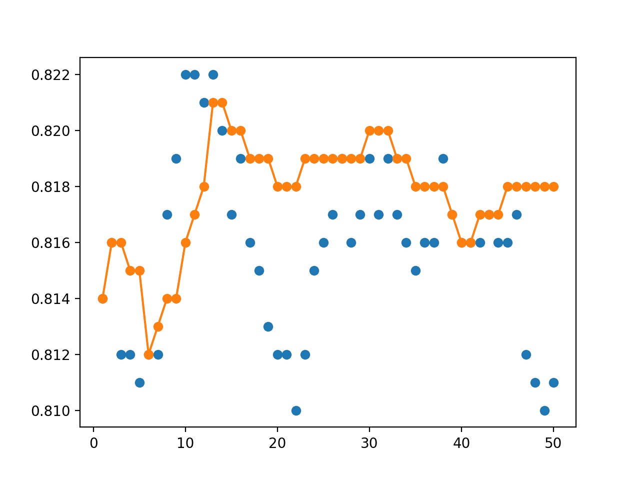
Line Plot Showing Single Model Accuracy (blue dots) vs Accuracy of Ensembles of Varying Size With a Horizontal Voting Ensemble
Extensions
This section lists some ideas for extending the tutorial that you may wish to explore.
- Dataset Size. Repeat the experiments with a smaller or larger sized dataset with a similar ratio of training to test examples.
- Larger Ensemble. Re-run the example with hundreds of final models and report the impact of the large ensemble sizes of accuracy on the test set.
- Random Sampling of Models. Re-run the example and compare the performance of ensembles of the same size with models saved over contiguous epochs to a random selection of saved models.
If you explore any of these extensions, I’d love to know.
Further Reading
This section provides more resources on the topic if you are looking to go deeper.
Papers
API
- Getting started with the Keras Sequential model
- Keras Core Layers API
- scipy.stats.mode API
- numpy.argmax API
- sklearn.datasets.make_blobs API
- How can I save a Keras model?
- Keras Callbacks API
Summary
In this tutorial, you discovered how to reduce the variance of a final deep learning neural network model using a horizontal voting ensemble.
Specifically, you learned:
- It is challenging to choose a final neural network model that has high variance on a training dataset.
- Horizontal voting ensembles provide a way to reduce variance and improve average model performance for models with high variance using a single training run.
- How to develop a horizontal voting ensemble in Python using Keras to improve the performance of a final multilayer Perceptron model for multi-class classification.
Do you have any questions?
Ask your questions in the comments below and I will do my best to answer.
The post How to Reduce Variance in the Final Deep Learning Model With a Horizontal Voting Ensemble appeared first on Machine Learning Mastery.