
Author: Jason Brownlee
The training process of neural networks is a challenging optimization process that can often fail to converge.
This can mean that the model at the end of training may not be a stable or best-performing set of weights to use as a final model.
One approach to address this problem is to use an average of the weights from multiple models seen toward the end of the training run. This is called Polyak-Ruppert averaging and can be further improved by using a linearly or exponentially decreasing weighted average of the model weights. In addition to resulting in a more stable model, the performance of the averaged model weights can also result in better performance.
In this tutorial, you will discover how to combine the weights from multiple different models into a single model for making predictions.
After completing this tutorial, you will know:
- The stochastic and challenging nature of training neural networks can mean that the optimization process does not converge.
- Creating a model with the average of the weights from models observed towards the end of a training run can result in a more stable and sometimes better-performing solution.
- How to develop final models created with the equal, linearly, and exponentially weighted average of model parameters from multiple saved models.
Let’s get started.

How to Create an Equally, Linearly, and Exponentially Weighted Average of Neural Network Model Weights in Keras
Photo by netselesoobrazno, some rights reserved.
Tutorial Overview
This tutorial is divided into seven parts; they are:
- Average Model Weight Ensemble
- Multi-Class Classification Problem
- Multilayer Perceptron Model
- Save Multiple Models to File
- New Model With Average Model Weights
- Predicting With an Average Model Weight Ensemble
- Linearly and Exponentially Decreasing Weighted Average
Average Model Weight Ensemble
Learning the weights for a deep neural network model requires solving a high-dimensional non-convex optimization problem.
A challenge with solving this optimization problem is that there are many “good” solutions and it is possible for the learning algorithm to bounce around and fail to settle in on one. In the area of stochastic optimization, this is referred to as problems with the convergence of the optimization algorithm on a solution, where a solution is defined by a set of specific weight values.
A symptom you may see if you have a problem with the convergence of your model is train and/or test loss value that shows higher than expected variance, e.g. it thrashes or bounces up and down over training epochs.
One approach to address this problem is to combine the weights collected towards the end of the training process. Generally, this might be referred to as temporal averaging and is known as Polyak Averaging or Polyak-Ruppert averaging, named for the original developers of the method.
Polyak averaging consists of averaging together several points in the trajectory through parameter space visited by an optimization algorithm.
— Page 322, Deep Learning, 2016.
Averaging multiple noisy sets of weights during the learning process may paradoxically sound less desirable than tuning the optimization process itself, but may prove a desirable solution, especially for very large neural networks that may take days, weeks, or even months to train.
The essential advancement was reached on the basis of the paradoxical idea: a slow algorithm having less than optimal convergence rate must be averaged.
— Acceleration of Stochastic Approximation by Averaging, 1992.
Averaging the weights of multiple models from a single training run has the effect of calming down the noisy optimization process that may be noisy because of the choice of learning hyperparameters (e.g. learning rate) or the shape of the mapping function that is being learned. The result is a final model or set of weights that may offer a more stable, and perhaps more accurate result.
The basic idea is that the optimization algorithm may leap back and forth across a valley several times without ever visiting a point near the bottom of the valley. The average of all of the locations on either side should be close to the bottom of the valley though.
— Page 322, Deep Learning, 2016.
The simplest implementation of Polyak-Ruppert averaging involves calculating the average of the weights of the models over the last few training epochs.
This can be improved by calculating a weighted average, where more weight is applied to more recent models, which is linearly decreased through prior epochs. An alternative and more widely used approach is to use an exponential decay in the weighted average.
Polyak-Ruppert averaging has been shown to improve the convergence of standard SGD […] . Alternatively, an exponential moving average over the parameters can be used, giving higher weight to more recent parameter value.
— Adam: A Method for Stochastic Optimization, 2014.
Using an average or weighted average of model weights in the final model is a common technique in practice for ensuring the very best results are achieved from the training run. The approach is one of many “tricks” used in the Google Inception V2 and V3 deep convolutional neural network models for photo classification, a milestone in the field of deep learning.
Model evaluations are performed using a running average of the parameters computed over time.
— Rethinking the Inception Architecture for Computer Vision, 2015.
Want Better Results with Deep Learning?
Take my free 7-day email crash course now (with sample code).
Click to sign-up and also get a free PDF Ebook version of the course.
Multi-Class Classification Problem
We will use a small multi-class classification problem as the basis to demonstrate the model weight ensemble.
The scikit-learn class provides the make_blobs() function that can be used to create a multi-class classification problem with the prescribed number of samples, input variables, classes, and variance of samples within a class.
The problem has two input variables (to represent the x and y coordinates of the points) and a standard deviation of 2.0 for points within each group. We will use the same random state (seed for the pseudorandom number generator) to ensure that we always get the same data points.
# generate 2d classification dataset
X, y = make_blobs(n_samples=1000, centers=3, n_features=2, cluster_std=2, random_state=2)
The results are the input and output elements of a dataset that we can model.
In order to get a feeling for the complexity of the problem, we can plot each point on a two-dimensional scatter plot and color each point by class value.
The complete example is listed below.
# scatter plot of blobs dataset
from sklearn.datasets.samples_generator import make_blobs
from matplotlib import pyplot
from numpy import where
# generate 2d classification dataset
X, y = make_blobs(n_samples=1000, centers=3, n_features=2, cluster_std=2, random_state=2)
# scatter plot for each class value
for class_value in range(3):
	# select indices of points with the class label
	row_ix = where(y == class_value)
	# scatter plot for points with a different color
	pyplot.scatter(X[row_ix, 0], X[row_ix, 1])
# show plot
pyplot.show()
Running the example creates a scatter plot of the entire dataset. We can see that the standard deviation of 2.0 means that the classes are not linearly separable (separable by a line) causing many ambiguous points.
This is desirable as it means that the problem is non-trivial and will allow a neural network model to find many different “good enough” candidate solutions resulting in a high variance.
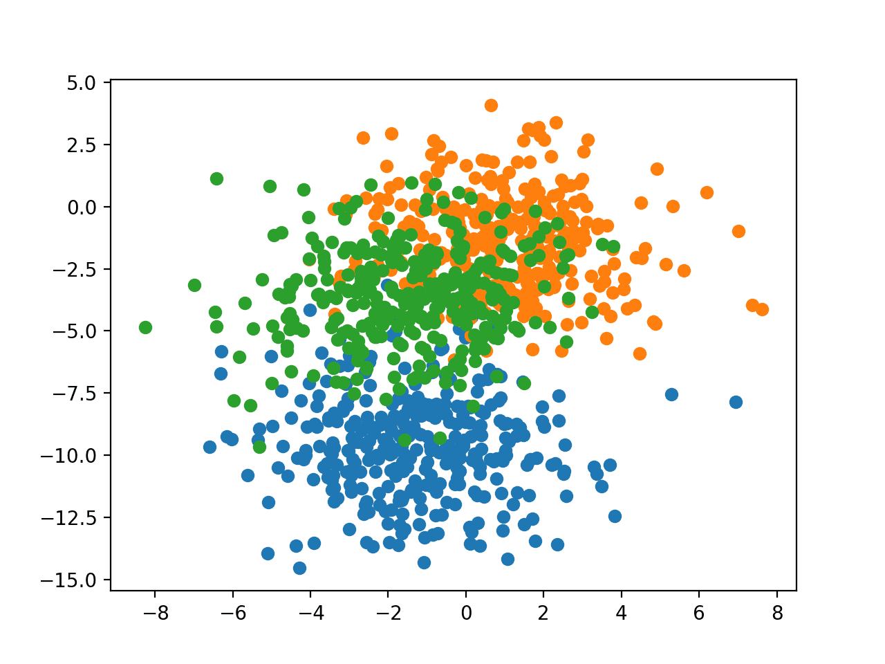
Scatter Plot of Blobs Dataset With Three Classes and Points Colored by Class Value
Multilayer Perceptron Model
Before we define a model, we need to contrive a problem that is appropriate for the ensemble.
In our problem, the training dataset is relatively small. Specifically, there is a 10:1 ratio of examples in the training dataset to the holdout dataset. This mimics a situation where we may have a vast number of unlabeled examples and a small number of labeled examples with which to train a model.
We will create 1,100 data points from the blobs problem. The model will be trained on the first 100 points and the remaining 1,000 will be held back in a test dataset, unavailable to the model.
The problem is a multi-class classification problem, and we will model it using a softmax activation function on the output layer. This means that the model will predict a vector with three elements with the probability that the sample belongs to each of the three classes. Therefore, we must one hot encode the class values before we split the rows into the train and test datasets. We can do this using the Keras to_categorical() function.
# generate 2d classification dataset
X, y = make_blobs(n_samples=1100, centers=3, n_features=2, cluster_std=2, random_state=2)
# one hot encode output variable
y = to_categorical(y)
# split into train and test
n_train = 100
trainX, testX = X[:n_train, :], X[n_train:, :]
trainy, testy = y[:n_train], y[n_train:]
Next, we can define and compile the model.
The model will expect samples with two input variables. The model then has a single hidden layer with 25 nodes and a rectified linear activation function, then an output layer with three nodes to predict the probability of each of the three classes and a softmax activation function.
Because the problem is multi-class, we will use the categorical cross entropy loss function to optimize the model and stochastic gradient descent with a small learning rate and momentum.
# define model
model = Sequential()
model.add(Dense(25, input_dim=2, activation='relu'))
model.add(Dense(3, activation='softmax'))
opt = SGD(lr=0.01, momentum=0.9)
model.compile(loss='categorical_crossentropy', optimizer=opt, metrics=['accuracy'])
The model is fit for 500 training epochs and we will evaluate the model each epoch on the test set, using the test set as a validation set.
# fit model
history = model.fit(trainX, trainy, validation_data=(testX, testy), epochs=500, verbose=0)
At the end of the run, we will evaluate the performance of the model on the train and test sets.
# evaluate the model
_, train_acc = model.evaluate(trainX, trainy, verbose=0)
_, test_acc = model.evaluate(testX, testy, verbose=0)
print('Train: %.3f, Test: %.3f' % (train_acc, test_acc))
Then finally, we will plot learning curves of the model accuracy over each training epoch on both the training and validation datasets.
# learning curves of model accuracy
pyplot.plot(history.history['acc'], label='train')
pyplot.plot(history.history['val_acc'], label='test')
pyplot.legend()
pyplot.show()
Tying all of this together, the complete example is listed below.
# develop an mlp for blobs dataset
from sklearn.datasets.samples_generator import make_blobs
from keras.utils import to_categorical
from keras.models import Sequential
from keras.layers import Dense
from keras.optimizers import SGD
from matplotlib import pyplot
# generate 2d classification dataset
X, y = make_blobs(n_samples=1100, centers=3, n_features=2, cluster_std=2, random_state=2)
# one hot encode output variable
y = to_categorical(y)
# split into train and test
n_train = 100
trainX, testX = X[:n_train, :], X[n_train:, :]
trainy, testy = y[:n_train], y[n_train:]
# define model
model = Sequential()
model.add(Dense(25, input_dim=2, activation='relu'))
model.add(Dense(3, activation='softmax'))
opt = SGD(lr=0.01, momentum=0.9)
model.compile(loss='categorical_crossentropy', optimizer=opt, metrics=['accuracy'])
# fit model
history = model.fit(trainX, trainy, validation_data=(testX, testy), epochs=500, verbose=0)
# evaluate the model
_, train_acc = model.evaluate(trainX, trainy, verbose=0)
_, test_acc = model.evaluate(testX, testy, verbose=0)
print('Train: %.3f, Test: %.3f' % (train_acc, test_acc))
# learning curves of model accuracy
pyplot.plot(history.history['acc'], label='train')
pyplot.plot(history.history['val_acc'], label='test')
pyplot.legend()
pyplot.show()
Running the example prints the performance of the final model on the train and test datasets.
Your specific results will vary (by design!) given the high variance nature of the model.
In this case, we can see that the model achieved about 86% accuracy on the training dataset, which we know is optimistic, and about 81% on the test dataset, which we would expect to be more realistic.
Train: 0.860, Test: 0.812
A line plot is also created showing the learning curves for the model accuracy on the train and test sets over each training epoch.
We can see that training accuracy is more optimistic over most of the run, as we also noted with the final scores. Importantly, we do see a reasonable amount of variance in the accuracy during training on both the train and test datasets, potentially providing a good basis for using model weight averaging.
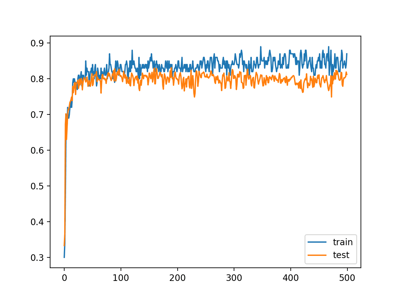
Line Plot Learning Curves of Model Accuracy on Train and Test Dataset over Each Training Epoch
Save Multiple Models to File
One approach to the model weight ensemble is to keep a running average of model weights in memory.
There are three downsides to this approach:
- It requires that you know beforehand the way in which the model weights will be combined; perhaps you want to experiment with different approaches.
- It requires that you know the number of epochs to use for training; maybe you want to use early stopping.
- It requires that you keep at least one copy of the entire network in memory; this could be very expensive for large models and fragile if the training process crashes or is killed.
An alternative is to save model weights to file during training as a first step, and later combine the weights from the saved models in order to make a final model.
Perhaps the simplest way to implement this is to manually drive the training process, one epoch at a time, then save models at the end of the epoch if we have exceeded an upper limit on the number of epochs.
For example, with our test problem, we will train the model for 500 epochs and perhaps save models from epoch 490 onwards (e.g. between and including epochs 490 and 499).
# fit model
n_epochs, n_save_after = 500, 490
for i in range(n_epochs):
	# fit model for a single epoch
	model.fit(trainX, trainy, epochs=1, verbose=0)
	# check if we should save the model
	if i >= n_save_after:
		model.save('model_' + str(i) + '.h5')
Models can be saved to file using the save() function on the model and specifying a filename that includes the epoch number.
Note, saving and loading neural network models in Keras requires that you have the h5py library installed. You can install this library using pip as follows:
pip install h5py
Tying all of this together, the complete example of fitting the model on the training dataset and saving all models from the last 10 epochs is listed below.
# save models to file toward the end of a training run
from sklearn.datasets.samples_generator import make_blobs
from keras.utils import to_categorical
from keras.models import Sequential
from keras.layers import Dense
# generate 2d classification dataset
X, y = make_blobs(n_samples=1100, centers=3, n_features=2, cluster_std=2, random_state=2)
# one hot encode output variable
y = to_categorical(y)
# split into train and test
n_train = 100
trainX, testX = X[:n_train, :], X[n_train:, :]
trainy, testy = y[:n_train], y[n_train:]
# define model
model = Sequential()
model.add(Dense(25, input_dim=2, activation='relu'))
model.add(Dense(3, activation='softmax'))
model.compile(loss='categorical_crossentropy', optimizer='adam', metrics=['accuracy'])
# fit model
n_epochs, n_save_after = 500, 490
for i in range(n_epochs):
	# fit model for a single epoch
	model.fit(trainX, trainy, epochs=1, verbose=0)
	# check if we should save the model
	if i >= n_save_after:
		model.save('model_' + str(i) + '.h5')
Running the example saves 10 models into the current working directory.
New Model With Average Models Weights
We can create a new model from multiple existing models with the same architecture.
First, we need to load the models into memory. This is reasonable as the models are small. If you are working with very large models, it might be easier to load models one at a time and average the weights in memory.
The load_model() Keras function can be used to load a saved model from file. The function load_all_models() below will load models from the current working directory. It takes the start and end epochs as arguments so that you can experiment with different groups of models saved over contiguous epochs.
# load models from file
def load_all_models(n_start, n_end):
	all_models = list()
	for epoch in range(n_start, n_end):
		# define filename for this ensemble
		filename = 'model_' + str(epoch) + '.h5'
		# load model from file
		model = load_model(filename)
		# add to list of members
		all_models.append(model)
		print('>loaded %s' % filename)
	return all_models
We can call the function to load all of the models.
# load models in order
members = load_all_models(490, 500)
print('Loaded %d models' % len(members))
Once loaded, we can create a new model with the weighted average of the model weights.
Each model has a get_weights() function that returns a list of arrays, one for each layer in the model. We can enumerate each layer in the model, retrieve the same layer from each model, and calculate the weighted average. This will give us a set of weights.
We can then use the clone_model() Keras function to create a clone of the architecture and call set_weights() function to use the average weights we have prepared. The model_weight_ensemble() function below implements this.
# create a model from the weights of multiple models
def model_weight_ensemble(members, weights):
	# determine how many layers need to be averaged
	n_layers = len(members[0].get_weights())
	# create an set of average model weights
	avg_model_weights = list()
	for layer in range(n_layers):
		# collect this layer from each model
		layer_weights = array([model.get_weights()[layer] for model in members])
		# weighted average of weights for this layer
		avg_layer_weights = average(layer_weights, axis=0, weights=weights)
		# store average layer weights
		avg_model_weights.append(avg_layer_weights)
	# create a new model with the same structure
	model = clone_model(members[0])
	# set the weights in the new
	model.set_weights(avg_model_weights)
	model.compile(loss='categorical_crossentropy', optimizer='adam', metrics=['accuracy'])
	return model
Tying these elements together, we can load the 10 models and calculate the equally weighted average (arithmetic average) of the model weights. The complete listing is provided below.
# average the weights of multiple loaded models
from keras.models import load_model
from keras.models import clone_model
from numpy import average
from numpy import array

# load models from file
def load_all_models(n_start, n_end):
	all_models = list()
	for epoch in range(n_start, n_end):
		# define filename for this ensemble
		filename = 'model_' + str(epoch) + '.h5'
		# load model from file
		model = load_model(filename)
		# add to list of members
		all_models.append(model)
		print('>loaded %s' % filename)
	return all_models

# create a model from the weights of multiple models
def model_weight_ensemble(members, weights):
	# determine how many layers need to be averaged
	n_layers = len(members[0].get_weights())
	# create an set of average model weights
	avg_model_weights = list()
	for layer in range(n_layers):
		# collect this layer from each model
		layer_weights = array([model.get_weights()[layer] for model in members])
		# weighted average of weights for this layer
		avg_layer_weights = average(layer_weights, axis=0, weights=weights)
		# store average layer weights
		avg_model_weights.append(avg_layer_weights)
	# create a new model with the same structure
	model = clone_model(members[0])
	# set the weights in the new
	model.set_weights(avg_model_weights)
	model.compile(loss='categorical_crossentropy', optimizer='adam', metrics=['accuracy'])
	return model

# load all models into memory
members = load_all_models(490, 500)
print('Loaded %d models' % len(members))
# prepare an array of equal weights
n_models = len(members)
weights = [1/n_models for i in range(1, n_models+1)]
# create a new model with the weighted average of all model weights
model = model_weight_ensemble(members, weights)
# summarize the created model
model.summary()
Running the example first loads the 10 models from file.
>loaded model_490.h5
>loaded model_491.h5
>loaded model_492.h5
>loaded model_493.h5
>loaded model_494.h5
>loaded model_495.h5
>loaded model_496.h5
>loaded model_497.h5
>loaded model_498.h5
>loaded model_499.h5
Loaded 10 models
A model weight ensemble is created from these 10 models giving equal weight to each model and a summary of the model structure is reported.
_________________________________________________________________
Layer (type)                 Output Shape              Param #
=================================================================
dense_1 (Dense)              (None, 25)                75
_________________________________________________________________
dense_2 (Dense)              (None, 3)                 78
=================================================================
Total params: 153
Trainable params: 153
Non-trainable params: 0
_________________________________________________________________
Predicting With an Average Model Weight Ensemble
Now that we know how to calculate a weighted average of model weights, we can evaluate predictions with the resulting model.
One issue is that we don’t know how many models are appropriate to combine in order to achieve good performance. We can address this by evaluating model weight averaging ensembles with the last n models and vary n to see how many models results in good performance.
The evaluate_n_members() function below will create a new model from a given number of loaded models. Each model is given an equal weight in contributing to the final model, then the model_weight_ensemble() function is called to create the final model that is then evaluated on the test dataset.
# evaluate a specific number of members in an ensemble
def evaluate_n_members(members, n_members, testX, testy):
	# reverse loaded models so we build the ensemble with the last models first
	members = list(reversed(members))
	# select a subset of members
	subset = members[:n_members]
	# prepare an array of equal weights
	weights = [1.0/n_members for i in range(1, n_members+1)]
	# create a new model with the weighted average of all model weights
	model = model_weight_ensemble(subset, weights)
	# make predictions and evaluate accuracy
	_, test_acc = model.evaluate(testX, testy, verbose=0)
	return test_acc
Importantly, the list of loaded models is reversed first to ensure that the last n models in the training run are used, which we would assume might have better performance on average.
# reverse loaded models so we build the ensemble with the last models first
members = list(reversed(members))
We can then evaluate models created from different numbers of the last n models saved from the training run from the last 1-model to the last 10 models. In addition to evaluating the combined final model, we can also evaluate each saved standalone model on the test dataset to compare performance.
# evaluate different numbers of ensembles on hold out set
single_scores, ensemble_scores = list(), list()
for i in range(1, len(members)+1):
	# evaluate model with i members
	ensemble_score = evaluate_n_members(members, i, testX, testy)
	# evaluate the i'th model standalone
	_, single_score = members[i-1].evaluate(testX, testy, verbose=0)
	# summarize this step
	print('> %d: single=%.3f, ensemble=%.3f' % (i, single_score, ensemble_score))
	ensemble_scores.append(ensemble_score)
	single_scores.append(single_score)
The collected scores can be plotted, with blue dots for the accuracy of the single saved models and the orange line for the test accuracy for the model that combines the weights the last n models.
# plot score vs number of ensemble members
x_axis = [i for i in range(1, len(members)+1)]
pyplot.plot(x_axis, single_scores, marker='o', linestyle='None')
pyplot.plot(x_axis, ensemble_scores, marker='o')
pyplot.show()
Tying all of this together, the complete example is listed below.
# average of model weights on blobs problem
from sklearn.datasets.samples_generator import make_blobs
from sklearn.metrics import accuracy_score
from keras.utils import to_categorical
from keras.models import load_model
from keras.models import clone_model
from keras.models import Sequential
from keras.layers import Dense
from matplotlib import pyplot
from numpy import average
from numpy import array

# load models from file
def load_all_models(n_start, n_end):
	all_models = list()
	for epoch in range(n_start, n_end):
		# define filename for this ensemble
		filename = 'model_' + str(epoch) + '.h5'
		# load model from file
		model = load_model(filename)
		# add to list of members
		all_models.append(model)
		print('>loaded %s' % filename)
	return all_models

# # create a model from the weights of multiple models
def model_weight_ensemble(members, weights):
	# determine how many layers need to be averaged
	n_layers = len(members[0].get_weights())
	# create an set of average model weights
	avg_model_weights = list()
	for layer in range(n_layers):
		# collect this layer from each model
		layer_weights = array([model.get_weights()[layer] for model in members])
		# weighted average of weights for this layer
		avg_layer_weights = average(layer_weights, axis=0, weights=weights)
		# store average layer weights
		avg_model_weights.append(avg_layer_weights)
	# create a new model with the same structure
	model = clone_model(members[0])
	# set the weights in the new
	model.set_weights(avg_model_weights)
	model.compile(loss='categorical_crossentropy', optimizer='adam', metrics=['accuracy'])
	return model

# evaluate a specific number of members in an ensemble
def evaluate_n_members(members, n_members, testX, testy):
	# select a subset of members
	subset = members[:n_members]
	# prepare an array of equal weights
	weights = [1.0/n_members for i in range(1, n_members+1)]
	# create a new model with the weighted average of all model weights
	model = model_weight_ensemble(subset, weights)
	# make predictions and evaluate accuracy
	_, test_acc = model.evaluate(testX, testy, verbose=0)
	return test_acc

# generate 2d classification dataset
X, y = make_blobs(n_samples=1100, centers=3, n_features=2, cluster_std=2, random_state=2)
# one hot encode output variable
y = to_categorical(y)
# split into train and test
n_train = 100
trainX, testX = X[:n_train, :], X[n_train:, :]
trainy, testy = y[:n_train], y[n_train:]
# load models in order
members = load_all_models(490, 500)
print('Loaded %d models' % len(members))
# reverse loaded models so we build the ensemble with the last models first
members = list(reversed(members))
# evaluate different numbers of ensembles on hold out set
single_scores, ensemble_scores = list(), list()
for i in range(1, len(members)+1):
	# evaluate model with i members
	ensemble_score = evaluate_n_members(members, i, testX, testy)
	# evaluate the i'th model standalone
	_, single_score = members[i-1].evaluate(testX, testy, verbose=0)
	# summarize this step
	print('> %d: single=%.3f, ensemble=%.3f' % (i, single_score, ensemble_score))
	ensemble_scores.append(ensemble_score)
	single_scores.append(single_score)
# plot score vs number of ensemble members
x_axis = [i for i in range(1, len(members)+1)]
pyplot.plot(x_axis, single_scores, marker='o', linestyle='None')
pyplot.plot(x_axis, ensemble_scores, marker='o')
pyplot.show()
Running the example first loads the 10 saved models.
>loaded model_490.h5
>loaded model_491.h5
>loaded model_492.h5
>loaded model_493.h5
>loaded model_494.h5
>loaded model_495.h5
>loaded model_496.h5
>loaded model_497.h5
>loaded model_498.h5
>loaded model_499.h5
Loaded 10 models
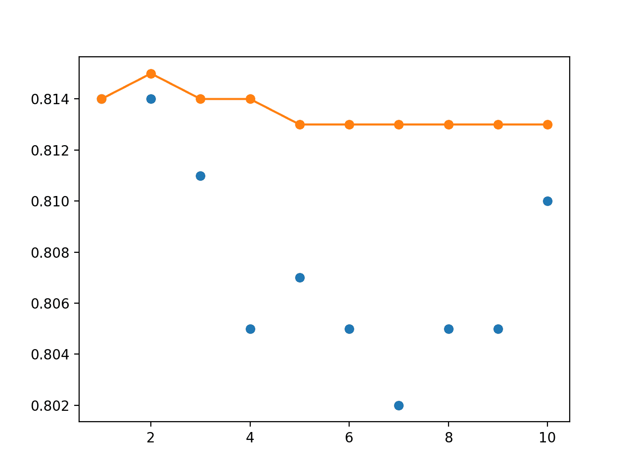
The performance of each individually saved model is reported as well as an ensemble model with weights averaged from all models up to and including each model, working backward from the end of the training run.
The results show that the best test accuracy was about 81.4% achieved by the last two models. We can see that the test accuracy of the model weight ensemble levels out the performance and performs just as well.
Your specific results will vary based on the models saved during the previous section.
> 1: single=0.814, ensemble=0.814
> 2: single=0.814, ensemble=0.814
> 3: single=0.811, ensemble=0.813
> 4: single=0.805, ensemble=0.813
> 5: single=0.807, ensemble=0.811
> 6: single=0.805, ensemble=0.807
> 7: single=0.802, ensemble=0.809
> 8: single=0.805, ensemble=0.808
> 9: single=0.805, ensemble=0.808
> 10: single=0.810, ensemble=0.807
A line plot is also created showing the test accuracy of each single model (blue dots) and the performance of the model weight ensemble (orange line).
We can see that averaging the model weights does level out the performance of the final model and performs at least as well as the final model of the run.
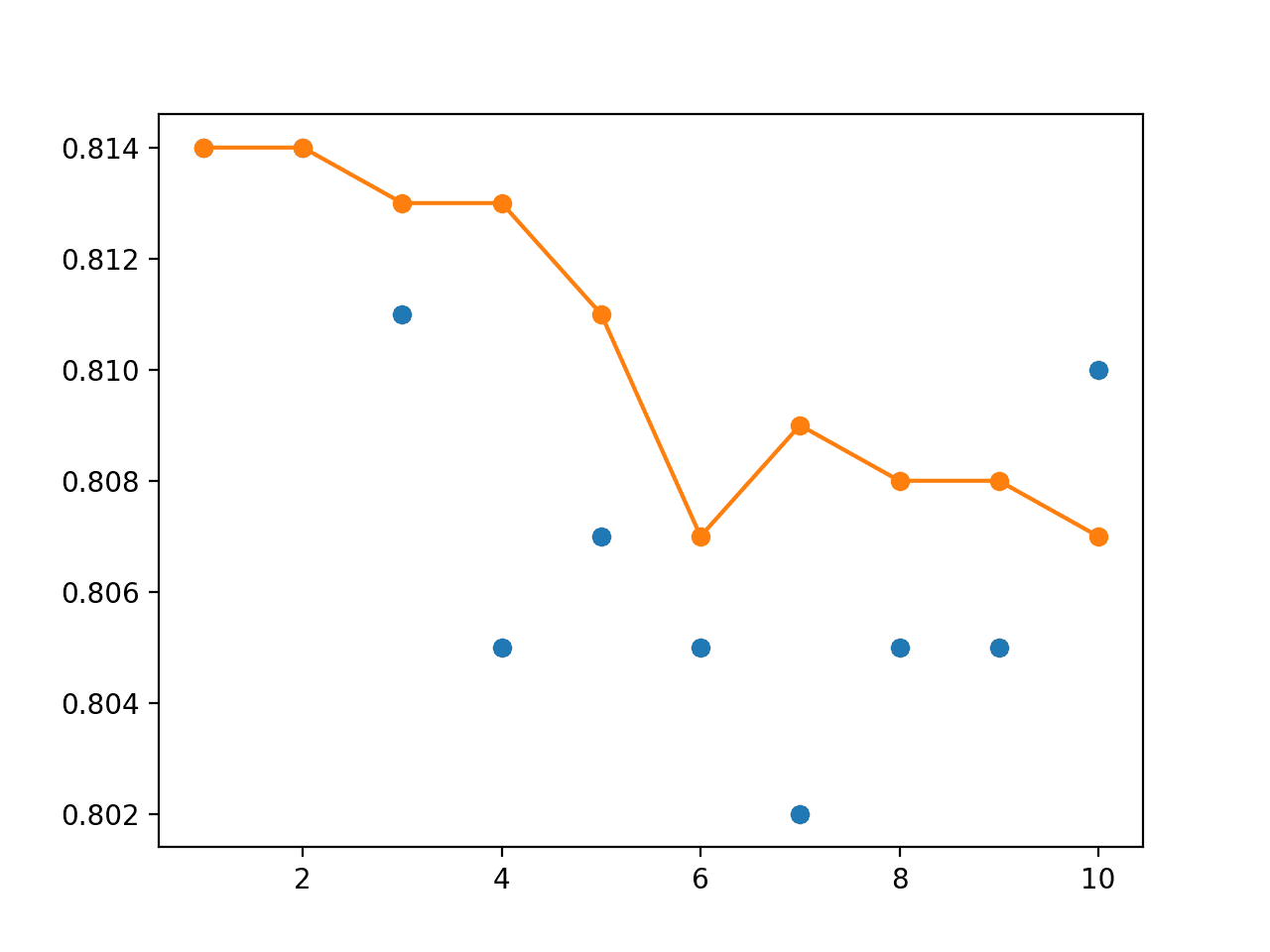
Line Plot of Single Model Test Performance (blue dots) and Model Weight Ensemble Test Performance (orange line)
Linearly and Exponentially Decreasing Weighted Average
We can update the example and evaluate a linearly decreasing weighting of the model weights in the ensemble.
The weights can be calculated as follows:
# prepare an array of linearly decreasing weights
weights = [i/n_members for i in range(n_members, 0, -1)]
This can be used instead of the equal weights in the evaluate_n_members() function.
The complete example is listed below.
# linearly decreasing weighted average of models on blobs problem
from sklearn.datasets.samples_generator import make_blobs
from sklearn.metrics import accuracy_score
from keras.utils import to_categorical
from keras.models import load_model
from keras.models import clone_model
from keras.models import Sequential
from keras.layers import Dense
from matplotlib import pyplot
from numpy import average
from numpy import array

# load models from file
def load_all_models(n_start, n_end):
	all_models = list()
	for epoch in range(n_start, n_end):
		# define filename for this ensemble
		filename = 'model_' + str(epoch) + '.h5'
		# load model from file
		model = load_model(filename)
		# add to list of members
		all_models.append(model)
		print('>loaded %s' % filename)
	return all_models

# create a model from the weights of multiple models
def model_weight_ensemble(members, weights):
	# determine how many layers need to be averaged
	n_layers = len(members[0].get_weights())
	# create an set of average model weights
	avg_model_weights = list()
	for layer in range(n_layers):
		# collect this layer from each model
		layer_weights = array([model.get_weights()[layer] for model in members])
		# weighted average of weights for this layer
		avg_layer_weights = average(layer_weights, axis=0, weights=weights)
		# store average layer weights
		avg_model_weights.append(avg_layer_weights)
	# create a new model with the same structure
	model = clone_model(members[0])
	# set the weights in the new
	model.set_weights(avg_model_weights)
	model.compile(loss='categorical_crossentropy', optimizer='adam', metrics=['accuracy'])
	return model

# evaluate a specific number of members in an ensemble
def evaluate_n_members(members, n_members, testX, testy):
	# select a subset of members
	subset = members[:n_members]
	# prepare an array of linearly decreasing weights
	weights = [i/n_members for i in range(n_members, 0, -1)]
	# create a new model with the weighted average of all model weights
	model = model_weight_ensemble(subset, weights)
	# make predictions and evaluate accuracy
	_, test_acc = model.evaluate(testX, testy, verbose=0)
	return test_acc

# generate 2d classification dataset
X, y = make_blobs(n_samples=1100, centers=3, n_features=2, cluster_std=2, random_state=2)
# one hot encode output variable
y = to_categorical(y)
# split into train and test
n_train = 100
trainX, testX = X[:n_train, :], X[n_train:, :]
trainy, testy = y[:n_train], y[n_train:]
# load models in order
members = load_all_models(490, 500)
print('Loaded %d models' % len(members))
# reverse loaded models so we build the ensemble with the last models first
members = list(reversed(members))
# evaluate different numbers of ensembles on hold out set
single_scores, ensemble_scores = list(), list()
for i in range(1, len(members)+1):
	# evaluate model with i members
	ensemble_score = evaluate_n_members(members, i, testX, testy)
	# evaluate the i'th model standalone
	_, single_score = members[i-1].evaluate(testX, testy, verbose=0)
	# summarize this step
	print('> %d: single=%.3f, ensemble=%.3f' % (i, single_score, ensemble_score))
	ensemble_scores.append(ensemble_score)
	single_scores.append(single_score)
# plot score vs number of ensemble members
x_axis = [i for i in range(1, len(members)+1)]
pyplot.plot(x_axis, single_scores, marker='o', linestyle='None')
pyplot.plot(x_axis, ensemble_scores, marker='o')
pyplot.show()
Running the example reports the performance of each single model again, and this time the test accuracy of each average model weight ensemble with a linearly decreasing contribution of models.
We can see that, at least in this case, the ensemble achieves a small bump in performance above any standalone model to about 81.5% accuracy.
...
> 1: single=0.814, ensemble=0.814
> 2: single=0.814, ensemble=0.815
> 3: single=0.811, ensemble=0.814
> 4: single=0.805, ensemble=0.813
> 5: single=0.807, ensemble=0.813
> 6: single=0.805, ensemble=0.813
> 7: single=0.802, ensemble=0.811
> 8: single=0.805, ensemble=0.810
> 9: single=0.805, ensemble=0.809
> 10: single=0.810, ensemble=0.809
The line plot shows the bump in performance and shows a more stable performance in terms of test accuracy over the different sized ensembles created, as compared to the use of an evenly weighted ensemble.
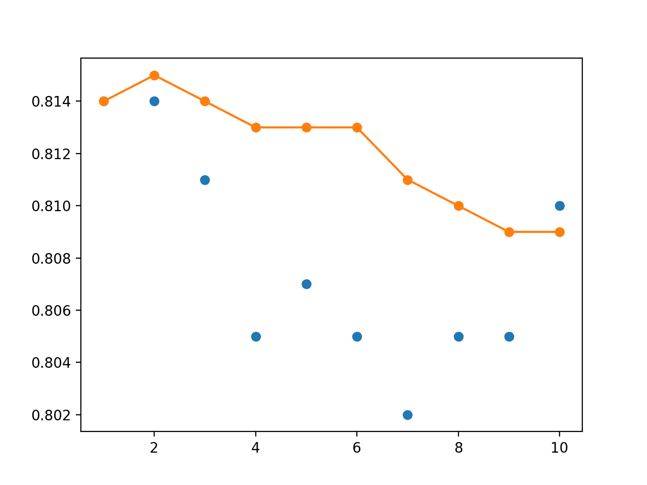
Line Plot of Single Model Test Performance (blue dots) and Model Weight Ensemble Test Performance (orange line) With a Linear Decay
We can also experiment with an exponential decay of the contribution of models. This requires that a decay rate (alpha) is specified. The example below creates weights for an exponential decay with a decrease rate of 2.
# prepare an array of exponentially decreasing weights
alpha = 2.0
weights = [exp(-i/alpha) for i in range(1, n_members+1)]
The complete example with an exponential decay for the contribution of models to the average weights in the ensemble model is listed below.
# exponentially decreasing weighted average of models on blobs problem
from sklearn.datasets.samples_generator import make_blobs
from sklearn.metrics import accuracy_score
from keras.utils import to_categorical
from keras.models import load_model
from keras.models import clone_model
from keras.models import Sequential
from keras.layers import Dense
from matplotlib import pyplot
from numpy import average
from numpy import array
from math import exp

# load models from file
def load_all_models(n_start, n_end):
	all_models = list()
	for epoch in range(n_start, n_end):
		# define filename for this ensemble
		filename = 'model_' + str(epoch) + '.h5'
		# load model from file
		model = load_model(filename)
		# add to list of members
		all_models.append(model)
		print('>loaded %s' % filename)
	return all_models

# create a model from the weights of multiple models
def model_weight_ensemble(members, weights):
	# determine how many layers need to be averaged
	n_layers = len(members[0].get_weights())
	# create an set of average model weights
	avg_model_weights = list()
	for layer in range(n_layers):
		# collect this layer from each model
		layer_weights = array([model.get_weights()[layer] for model in members])
		# weighted average of weights for this layer
		avg_layer_weights = average(layer_weights, axis=0, weights=weights)
		# store average layer weights
		avg_model_weights.append(avg_layer_weights)
	# create a new model with the same structure
	model = clone_model(members[0])
	# set the weights in the new
	model.set_weights(avg_model_weights)
	model.compile(loss='categorical_crossentropy', optimizer='adam', metrics=['accuracy'])
	return model

# evaluate a specific number of members in an ensemble
def evaluate_n_members(members, n_members, testX, testy):
	# select a subset of members
	subset = members[:n_members]
	# prepare an array of exponentially decreasing weights
	alpha = 2.0
	weights = [exp(-i/alpha) for i in range(1, n_members+1)]
	# create a new model with the weighted average of all model weights
	model = model_weight_ensemble(subset, weights)
	# make predictions and evaluate accuracy
	_, test_acc = model.evaluate(testX, testy, verbose=0)
	return test_acc

# generate 2d classification dataset
X, y = make_blobs(n_samples=1100, centers=3, n_features=2, cluster_std=2, random_state=2)
# one hot encode output variable
y = to_categorical(y)
# split into train and test
n_train = 100
trainX, testX = X[:n_train, :], X[n_train:, :]
trainy, testy = y[:n_train], y[n_train:]
# load models in order
members = load_all_models(490, 500)
print('Loaded %d models' % len(members))
# reverse loaded models so we build the ensemble with the last models first
members = list(reversed(members))
# evaluate different numbers of ensembles on hold out set
single_scores, ensemble_scores = list(), list()
for i in range(1, len(members)+1):
	# evaluate model with i members
	ensemble_score = evaluate_n_members(members, i, testX, testy)
	# evaluate the i'th model standalone
	_, single_score = members[i-1].evaluate(testX, testy, verbose=0)
	# summarize this step
	print('> %d: single=%.3f, ensemble=%.3f' % (i, single_score, ensemble_score))
	ensemble_scores.append(ensemble_score)
	single_scores.append(single_score)
# plot score vs number of ensemble members
x_axis = [i for i in range(1, len(members)+1)]
pyplot.plot(x_axis, single_scores, marker='o', linestyle='None')
pyplot.plot(x_axis, ensemble_scores, marker='o')
pyplot.show()
Running the example shows a small improvement in performance much like the use of a linear decay in the weighted average of the saved models.
> 1: single=0.814, ensemble=0.814
> 2: single=0.814, ensemble=0.815
> 3: single=0.811, ensemble=0.814
> 4: single=0.805, ensemble=0.814
> 5: single=0.807, ensemble=0.813
> 6: single=0.805, ensemble=0.813
> 7: single=0.802, ensemble=0.813
> 8: single=0.805, ensemble=0.813
> 9: single=0.805, ensemble=0.813
> 10: single=0.810, ensemble=0.813
The line plot of the test accuracy scores shows the stronger stabilizing effect of using the exponential decay instead of the linear or equal weighting of models.
Line Plot of Single Model Test Performance (blue dots) and Model Weight Ensemble Test Performance (orange line) With an Exponential Decay
Extensions
This section lists some ideas for extending the tutorial that you may wish to explore.
- Number of Models. Evaluate the effect of many more models contributing their weights to the final model.
- Decay Rate. Evaluate the effect on test performance of using different decay rates for an exponentially weighted average.
If you explore any of these extensions, I’d love to know.
Further Reading
This section provides more resources on the topic if you are looking to go deeper.
Books
- Section 8.7.3 Polyak Averaging, Deep Learning, 2016.
Papers
- Acceleration of Stochastic Approximation by Averaging, 1992.
- Efficient estimations from a slowly convergent robbins-monro process, 1988.
API
- Getting started with the Keras Sequential model
- Keras Core Layers API
- sklearn.datasets.make_blobs API
- numpy.average API
Articles
- Average weights in keras models, StackOverflow.
- Model Ensembles, CS231n Convolutional Neural Networks for Visual Recognition
- Exponential Moving Average, Keras Issue.
- ExponentialMovingAverage Implementation
Summary
In this tutorial, you discovered how to combine the weights from multiple different models into a single model for making predictions.
Specifically, you learned:
- The stochastic and challenging nature of training neural networks can mean that the optimization process does not converge.
- Creating a model with the average of the weights from models observed towards the end of a training run can result in a more stable and sometimes better-performing solution.
- How to develop final models created with the equal, linearly, and exponentially weighted average of model parameters from multiple saved models.
Do you have any questions?
Ask your questions in the comments below and I will do my best to answer.
The post How to Create an Equally, Linearly, and Exponentially Weighted Average of Neural Network Model Weights in Keras appeared first on Machine Learning Mastery.