
Author: Jason Brownlee
Neural networks are trained using gradient descent where the estimate of the error used to update the weights is calculated based on a subset of the training dataset.
The number of examples from the training dataset used in the estimate of the error gradient is called the batch size and is an important hyperparameter that influences the dynamics of the learning algorithm.
It is important to explore the dynamics of your model to ensure that you’re getting the most out of it.
In this tutorial, you will discover three different flavors of gradient descent and how to explore and diagnose the effect of batch size on the learning process.
After completing this tutorial, you will know:
- Batch size controls the accuracy of the estimate of the error gradient when training neural networks.
- Batch, Stochastic, and Minibatch gradient descent are the three main flavors of the learning algorithm.
- There is a tension between batch size and the speed and stability of the learning process.
Let’s get started.

How to Control the Speed and Stability of Training Neural Networks With Gradient Descent Batch Size
Photo by Adrian Scottow, some rights reserved.
Tutorial Overview
This tutorial is divided into seven parts; they are:
- Batch Size and Gradient Descent
- Stochastic, Batch, and Minibatch Gradient Descent in Keras
- Multi-Class Classification Problem
- MLP Fit With Batch Gradient Descent
- MLP Fit With Stochastic Gradient Descent
- MLP Fit With Minibatch Gradient Descent
- Effect of Batch Size on Model Behavior
Batch Size and Gradient Descent
Neural networks are trained using the stochastic gradient descent optimization algorithm.
This involves using the current state of the model to make a prediction, comparing the prediction to the expected values, and using the difference as an estimate of the error gradient. This error gradient is then used to update the model weights and the process is repeated.
The error gradient is a statistical estimate. The more training examples used in the estimate, the more accurate this estimate will be and the more likely that the weights of the network will be adjusted in a way that will improve the performance of the model. The improved estimate of the error gradient comes at the cost of having to use the model to make many more predictions before the estimate can be calculated, and in turn, the weights updated.
Optimization algorithms that use the entire training set are called batch or deterministic gradient methods, because they process all of the training examples simultaneously in a large batch.
— Page 278, Deep Learning, 2016.
Alternately, using fewer examples results in a less accurate estimate of the error gradient that is highly dependent on the specific training examples used.
This results in a noisy estimate that, in turn, results in noisy updates to the model weights, e.g. many updates with perhaps quite different estimates of the error gradient. Nevertheless, these noisy updates can result in faster learning and sometimes a more robust model.
Optimization algorithms that use only a single example at a time are sometimes called stochastic or sometimes online methods. The term online is usually reserved for the case where the examples are drawn from a stream of continually created examples rather than from a fixed-size training set over which several passes are made.
— Page 278, Deep Learning, 2016.
The number of training examples used in the estimate of the error gradient is a hyperparameter for the learning algorithm called the “batch size,” or simply the “batch.”
A batch size of 32 means that 32 samples from the training dataset will be used to estimate the error gradient before the model weights are updated. One training epoch means that the learning algorithm has made one pass through the training dataset, where examples were separated into randomly selected “batch size” groups.
Historically, a training algorithm where the batch size is set to the total number of training examples is called “batch gradient descent” and a training algorithm where the batch size is set to 1 training example is called “stochastic gradient descent” or “online gradient descent.”
A configuration of the batch size anywhere in between (e.g. more than 1 example and less than the number of examples in the training dataset) is called “minibatch gradient descent.”
- Batch Gradient Descent. Batch size is set to the total number of examples in the training dataset.
- Stochastic Gradient Descent. Batch size is set to one.
- Minibatch Gradient Descent. Batch size is set to more than one and less than the total number of examples in the training dataset.
For shorthand, the algorithm is often referred to as stochastic gradient descent regardless of the batch size. Given that very large datasets are often used to train deep learning neural networks, the batch size is rarely set to the size of the training dataset.
Smaller batch sizes are used for two main reasons:
- Smaller batch sizes are noisy, offering a regularizing effect and lower generalization error.
- Smaller batch sizes make it easier to fit one batch worth of training data in memory (i.e. when using a GPU).
A third reason is that the batch size is often set at something small, such as 32 examples, and is not tuned by the practitioner. Small batch sizes such as 32 do work well generally.
… [batch size] is typically chosen between 1 and a few hundreds, e.g. [batch size] = 32 is a good default value
— Practical recommendations for gradient-based training of deep architectures, 2012.
The presented results confirm that using small batch sizes achieves the best training stability and generalization performance, for a given computational cost, across a wide range of experiments. In all cases the best results have been obtained with batch sizes m = 32 or smaller, often as small as m = 2 or m = 4.
— Revisiting Small Batch Training for Deep Neural Networks, 2018.
Nevertheless, the batch size impacts how quickly a model learns and the stability of the learning process. It is an important hyperparameter that should be well understood and tuned by the deep learning practitioner.
Want Better Results with Deep Learning?
Take my free 7-day email crash course now (with sample code).
Click to sign-up and also get a free PDF Ebook version of the course.
Stochastic, Batch, and Minibatch Gradient Descent in Keras
Keras allows you to train your model using stochastic, batch, or minibatch gradient descent.
This can be achieved by setting the batch_size argument on the call to the fit() function when training your model.
Let’s take a look at each approach in turn.
Stochastic Gradient Descent in Keras
The example below sets the batch_size argument to 1 for stochastic gradient descent.
...
model.fit(trainX, trainy, batch_size=1)
Batch Gradient Descent in Keras
The example below sets the batch_size argument to the number of samples in the training dataset for batch gradient descent.
...
model.fit(trainX, trainy, batch_size=len(trainX))
Minibatch Gradient Descent in Keras
The example below uses the default batch size of 32 for the batch_size argument, which is more than 1 for stochastic gradient descent and less that the size of your training dataset for batch gradient descent.
...
model.fit(trainX, trainy)
Alternately, the batch_size can be specified to something other than 1 or the number of samples in the training dataset, such as 64.
...
model.fit(trainX, trainy, batch_size=64)
Multi-Class Classification Problem
We will use a small multi-class classification problem as the basis to demonstrate the effect of batch size on learning.
The scikit-learn class provides the make_blobs() function that can be used to create a multi-class classification problem with the prescribed number of samples, input variables, classes, and variance of samples within a class.
The problem can be configured to have two input variables (to represent the x and y coordinates of the points) and a standard deviation of 2.0 for points within each group. We will use the same random state (seed for the pseudorandom number generator) to ensure that we always get the same data points.
# generate 2d classification dataset
X, y = make_blobs(n_samples=1000, centers=3, n_features=2, cluster_std=2, random_state=2)
The results are the input and output elements of a dataset that we can model.
In order to get a feeling for the complexity of the problem, we can plot each point on a two-dimensional scatter plot and color each point by class value.
The complete example is listed below.
# scatter plot of blobs dataset
from sklearn.datasets.samples_generator import make_blobs
from matplotlib import pyplot
from numpy import where
# generate 2d classification dataset
X, y = make_blobs(n_samples=1000, centers=3, n_features=2, cluster_std=2, random_state=2)
# scatter plot for each class value
for class_value in range(3):
	# select indices of points with the class label
	row_ix = where(y == class_value)
	# scatter plot for points with a different color
	pyplot.scatter(X[row_ix, 0], X[row_ix, 1])
# show plot
pyplot.show()
Running the example creates a scatter plot of the entire dataset. We can see that the standard deviation of 2.0 means that the classes are not linearly separable (separable by a line) causing many ambiguous points.
This is desirable as it means that the problem is non-trivial and will allow a neural network model to find many different “good enough” candidate solutions.
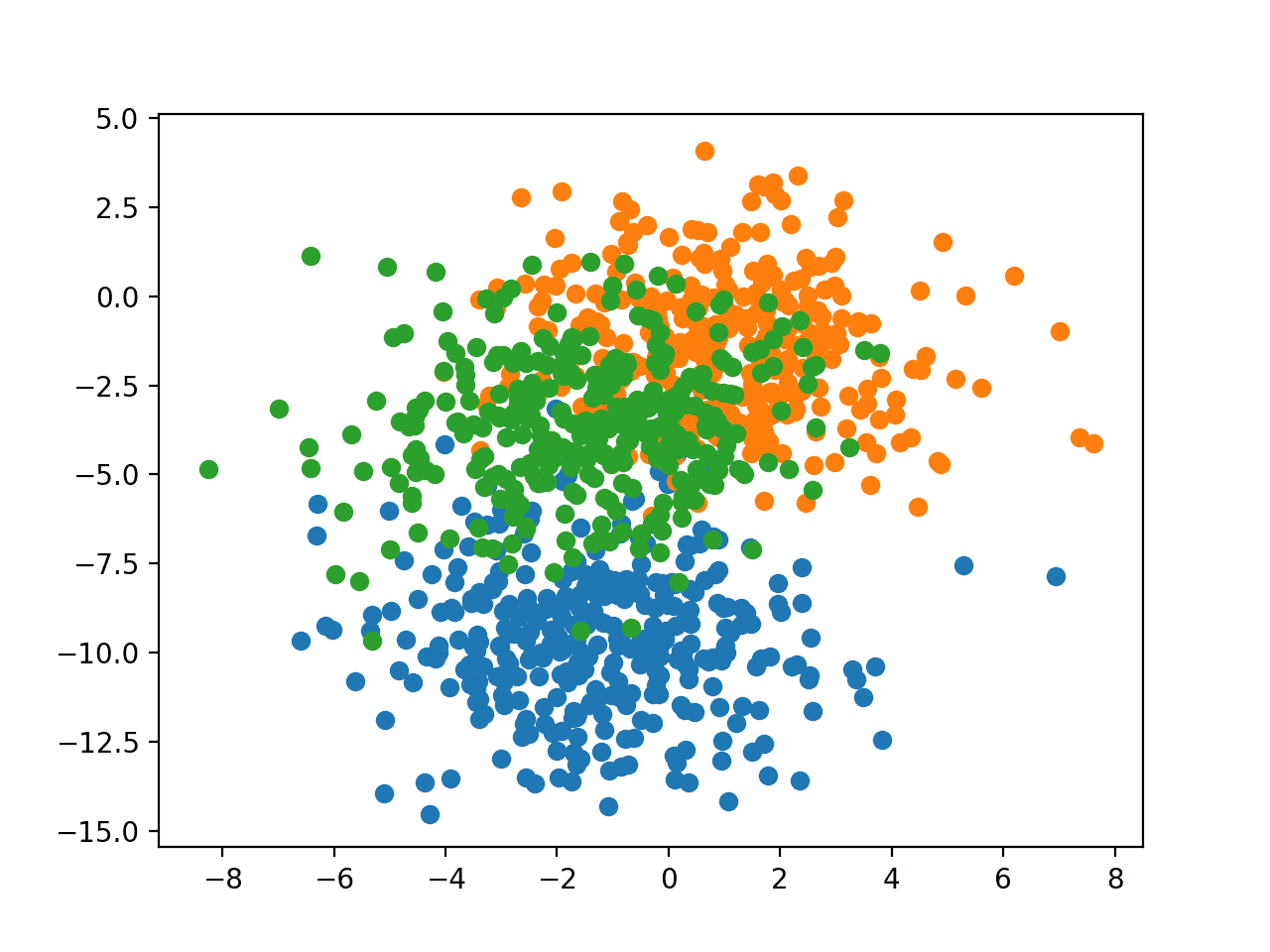
Scatter Plot of Blobs Dataset With Three Classes and Points Colored by Class Value
MLP Fit With Batch Gradient Descent
We can develop a Multilayer Perceptron model (MLP) to address the multi-class classification problem described in the previous section and train it using batch gradient descent.
Firstly, we need to one hot encode the target variable, transforming the integer class values into binary vectors. This will allow the model to predict the probability of each example belonging to each of the three classes, providing more nuance in the predictions and context when training the model.
# one hot encode output variable
y = to_categorical(y)
Next, we will split the training dataset of 1,000 examples into a train and test dataset with 500 examples each.
This even split will allow us to evaluate and compare the performance of different configurations of the batch size on the model and its performance.
# split into train and test
n_train = 500
trainX, testX = X[:n_train, :], X[n_train:, :]
trainy, testy = y[:n_train], y[n_train:]
We will define an MLP model with an input layer that expects two input variables, for the two variables in the dataset.
The model will have a single hidden layer with 50 nodes and a rectified linear activation function and He random weight initialization. Finally, the output layer has 3 nodes in order to make predictions for the three classes and a softmax activation function.
# define model
model = Sequential()
model.add(Dense(50, input_dim=2, activation='relu', kernel_initializer='he_uniform'))
model.add(Dense(3, activation='softmax'))
We will optimize the model with stochastic gradient descent and use categorical cross entropy to calculate the error of the model during training.
In this example, we will use “batch gradient descent“, meaning that the batch size will be set to the size of the training dataset. The model will be fit for 200 training epochs and the test dataset will be used as the validation set in order to monitor the performance of the model on a holdout set during training.
The effect will be more time between weight updates and we would expect faster training than other batch sizes, and more stable estimates of the gradient, which should result in a more stable performance of the model during training.
# compile model
opt = SGD(lr=0.01, momentum=0.9)
model.compile(loss='categorical_crossentropy', optimizer=opt, metrics=['accuracy'])
# fit model
history = model.fit(trainX, trainy, validation_data=(testX, testy), epochs=200, verbose=0, batch_size=len(trainX))
Once the model is fit, the performance is evaluated and reported on the train and test datasets.
# evaluate the model
_, train_acc = model.evaluate(trainX, trainy, verbose=0)
_, test_acc = model.evaluate(testX, testy, verbose=0)
print('Train: %.3f, Test: %.3f' % (train_acc, test_acc))
A line plot is created showing the train and test set accuracy of the model for each training epoch.
These learning curves provide an indication of three things: how quickly the model learns the problem, how well it has learned the problem, and how noisy the updates were to the model during training.
# plot training history
pyplot.plot(history.history['acc'], label='train')
pyplot.plot(history.history['val_acc'], label='test')
pyplot.legend()
pyplot.show()
Tying these elements together, the complete example is listed below.
# mlp for the blobs problem with batch gradient descent
from sklearn.datasets.samples_generator import make_blobs
from keras.layers import Dense
from keras.models import Sequential
from keras.optimizers import SGD
from keras.utils import to_categorical
from matplotlib import pyplot
# generate 2d classification dataset
X, y = make_blobs(n_samples=1000, centers=3, n_features=2, cluster_std=2, random_state=2)
# one hot encode output variable
y = to_categorical(y)
# split into train and test
n_train = 500
trainX, testX = X[:n_train, :], X[n_train:, :]
trainy, testy = y[:n_train], y[n_train:]
# define model
model = Sequential()
model.add(Dense(50, input_dim=2, activation='relu', kernel_initializer='he_uniform'))
model.add(Dense(3, activation='softmax'))
# compile model
opt = SGD(lr=0.01, momentum=0.9)
model.compile(loss='categorical_crossentropy', optimizer=opt, metrics=['accuracy'])
# fit model
history = model.fit(trainX, trainy, validation_data=(testX, testy), epochs=200, verbose=0, batch_size=len(trainX))
# evaluate the model
_, train_acc = model.evaluate(trainX, trainy, verbose=0)
_, test_acc = model.evaluate(testX, testy, verbose=0)
print('Train: %.3f, Test: %.3f' % (train_acc, test_acc))
# plot training history
pyplot.plot(history.history['acc'], label='train')
pyplot.plot(history.history['val_acc'], label='test')
pyplot.legend()
pyplot.show()
Running the example first reports the performance of the model on the train and test datasets.
Your specific results may vary given the stochastic nature of the learning algorithm; consider running the example a few times.
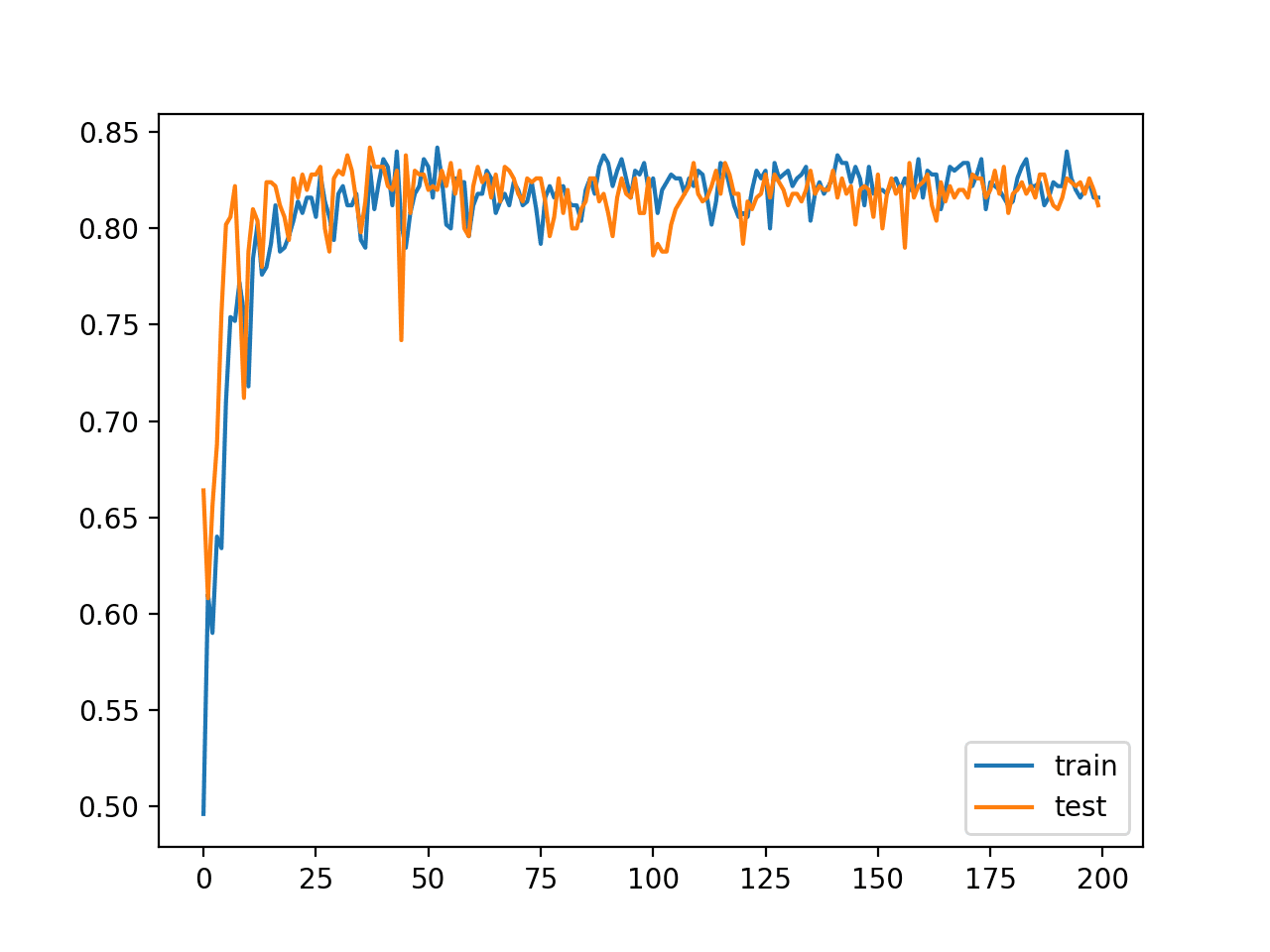
In this case, we can see that performance was similar between the train and test sets with 81% and 83% respectively.
Train: 0.816, Test: 0.830
A line plot of model classification accuracy on the train (blue) and test (orange) dataset is created. We can see that the model is relatively slow to learn this problem, converging on a solution after about 100 epochs after which changes in model performance are minor.
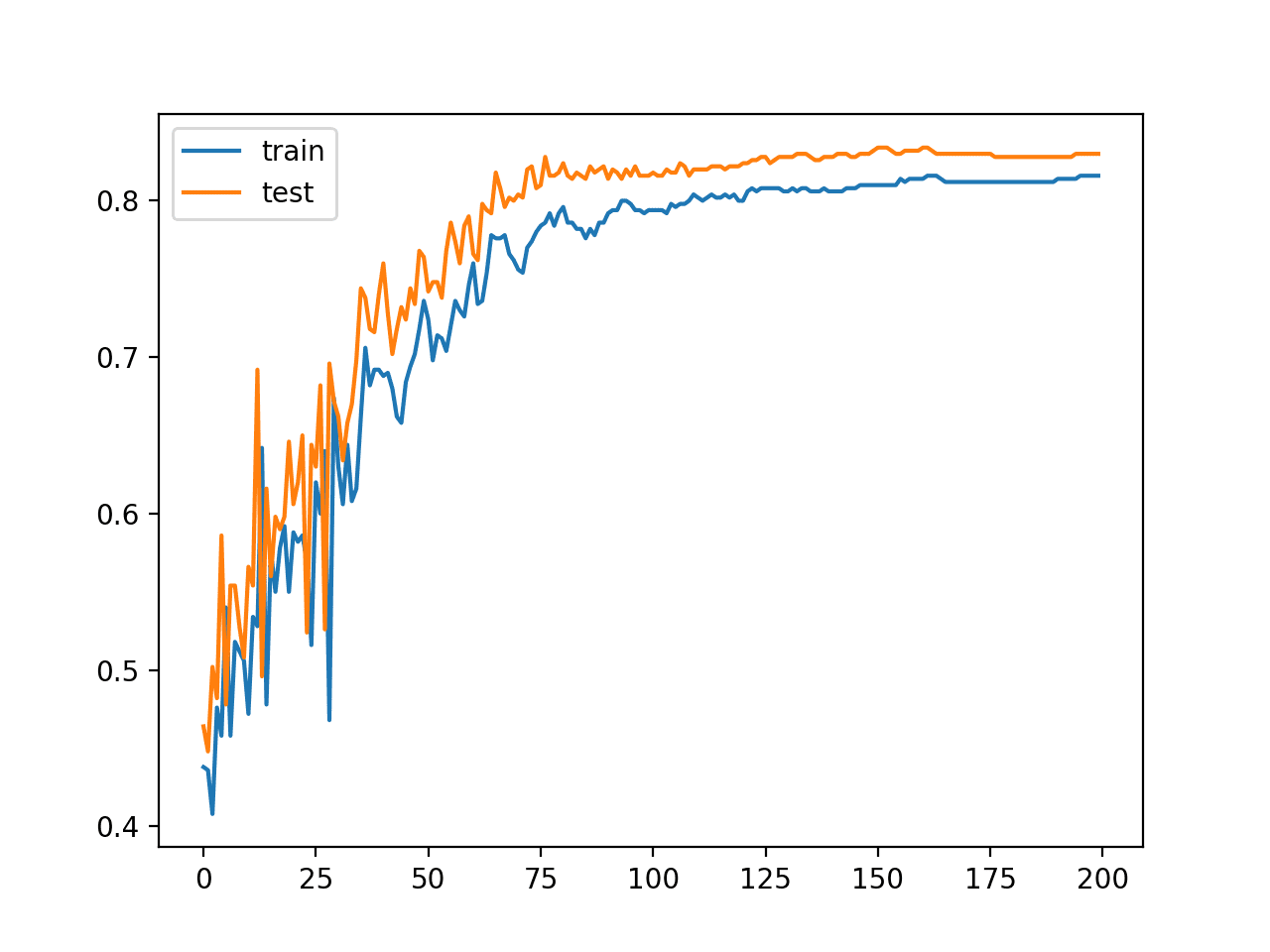
Line Plot of Classification Accuracy on Train and Tests Sets of an MLP Fit With Batch Gradient Descent
MLP Fit With Stochastic Gradient Descent
The example of batch gradient descent from the previous section can be updated to instead use stochastic gradient descent.
This requires changing the batch size from the size of the training dataset to 1.
# fit model
history = model.fit(trainX, trainy, validation_data=(testX, testy), epochs=200, verbose=0, batch_size=1)
Stochastic gradient descent requires that the model make a prediction and have the weights updated for each training example. This has the effect of dramatically slowing down the training process as compared to batch gradient descent.
The expectation of this change is that the model learns faster and that changes to the model are noisy, resulting, in turn, in noisy performance over training epochs.
The complete example with this change is listed below.
# mlp for the blobs problem with stochastic gradient descent
from sklearn.datasets.samples_generator import make_blobs
from keras.layers import Dense
from keras.models import Sequential
from keras.optimizers import SGD
from keras.utils import to_categorical
from matplotlib import pyplot
# generate 2d classification dataset
X, y = make_blobs(n_samples=1000, centers=3, n_features=2, cluster_std=2, random_state=2)
# one hot encode output variable
y = to_categorical(y)
# split into train and test
n_train = 500
trainX, testX = X[:n_train, :], X[n_train:, :]
trainy, testy = y[:n_train], y[n_train:]
# define model
model = Sequential()
model.add(Dense(50, input_dim=2, activation='relu', kernel_initializer='he_uniform'))
model.add(Dense(3, activation='softmax'))
# compile model
opt = SGD(lr=0.01, momentum=0.9)
model.compile(loss='categorical_crossentropy', optimizer=opt, metrics=['accuracy'])
# fit model
history = model.fit(trainX, trainy, validation_data=(testX, testy), epochs=200, verbose=0, batch_size=1)
# evaluate the model
_, train_acc = model.evaluate(trainX, trainy, verbose=0)
_, test_acc = model.evaluate(testX, testy, verbose=0)
print('Train: %.3f, Test: %.3f' % (train_acc, test_acc))
# plot training history
pyplot.plot(history.history['acc'], label='train')
pyplot.plot(history.history['val_acc'], label='test')
pyplot.legend()
pyplot.show()
Running the example first reports the performance of the model on the train and test datasets.
Your specific results may vary given the stochastic nature of the learning algorithm; consider running the example a few times.
In this case, we can see that performance was similar between the train and test sets, around 60% accuracy, but was dramatically worse (about 20 percentage points) than using batch gradient descent.
At least for this problem and the chosen model and model configuration, stochastic (online) gradient descent is not appropriate.
Train: 0.612, Test: 0.606
A line plot of model classification accuracy on the train (blue) and test (orange) dataset is created.
The plot shows the unstable nature of the training process with the chosen configuration. The poor performance and violent changes to the model suggest that the learning rate used to update weights after each training example may be too large and that a smaller learning rate may make the learning process more stable.
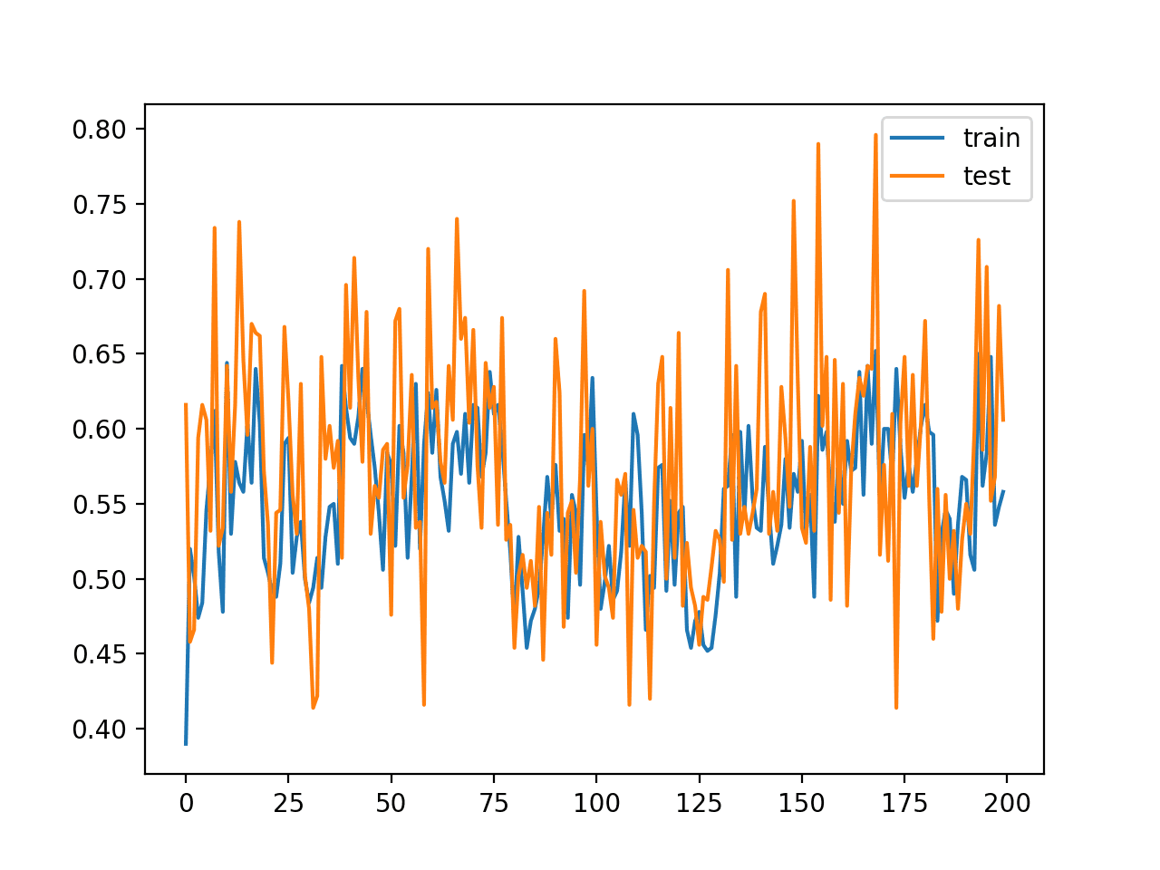
Line Plot of Classification Accuracy on Train and Tests Sets of an MLP Fit With Stochastic Gradient Descent
We can test this by re-running the model fit with stochastic gradient descent and a smaller learning rate. For example, we can drop the learning rate by an order of magnitude form 0.01 to 0.001.
# compile model
opt = SGD(lr=0.001, momentum=0.9)
model.compile(loss='categorical_crossentropy', optimizer=opt, metrics=['accuracy'])
The full code listing with this change is provided below for completeness.
# mlp for the blobs problem with stochastic gradient descent
from sklearn.datasets.samples_generator import make_blobs
from keras.layers import Dense
from keras.models import Sequential
from keras.optimizers import SGD
from keras.utils import to_categorical
from matplotlib import pyplot
# generate 2d classification dataset
X, y = make_blobs(n_samples=1000, centers=3, n_features=2, cluster_std=2, random_state=2)
# one hot encode output variable
y = to_categorical(y)
# split into train and test
n_train = 500
trainX, testX = X[:n_train, :], X[n_train:, :]
trainy, testy = y[:n_train], y[n_train:]
# define model
model = Sequential()
model.add(Dense(50, input_dim=2, activation='relu', kernel_initializer='he_uniform'))
model.add(Dense(3, activation='softmax'))
# compile model
opt = SGD(lr=0.001, momentum=0.9)
model.compile(loss='categorical_crossentropy', optimizer=opt, metrics=['accuracy'])
# fit model
history = model.fit(trainX, trainy, validation_data=(testX, testy), epochs=200, verbose=0, batch_size=1)
# evaluate the model
_, train_acc = model.evaluate(trainX, trainy, verbose=0)
_, test_acc = model.evaluate(testX, testy, verbose=0)
print('Train: %.3f, Test: %.3f' % (train_acc, test_acc))
# plot training history
pyplot.plot(history.history['acc'], label='train')
pyplot.plot(history.history['val_acc'], label='test')
pyplot.legend()
pyplot.show()
Running this example tells a very different story.
Your specific results may vary given the stochastic nature of the learning algorithm; consider running the example a few times.
The reported performance is greatly improved, achieving classification accuracy on the train and test sets on par with fit using batch gradient descent.
Train: 0.816, Test: 0.824
The line plot shows the expected behavior. Namely, that the model rapidly learns the problem as compared to batch gradient descent, leaping up to about 80% accuracy in about 25 epochs rather than the 100 epochs seen when using batch gradient descent. We could have stopped training at epoch 50 instead of epoch 200 due to the faster training.
This is not surprising. With batch gradient descent, 100 epochs involved 100 estimates of error and 100 weight updates. In stochastic gradient descent, 25 epochs involved (500 * 25) or 12,500 weight updates, providing more than 10-times more feedback, albeit more noisy feedback, about how to improve the model.
The line plot also shows that train and test performance remain comparable during training, as compared to the dynamics with batch gradient descent where the performance on the test set was slightly better and remained so throughout training.
Unlike batch gradient descent, we can see that the noisy updates result in noisy performance throughout the duration of training. This variance in the model means that it may be challenging to choose which model to use as the final model, as opposed to batch gradient descent where performance is stabilized because the model has converged.
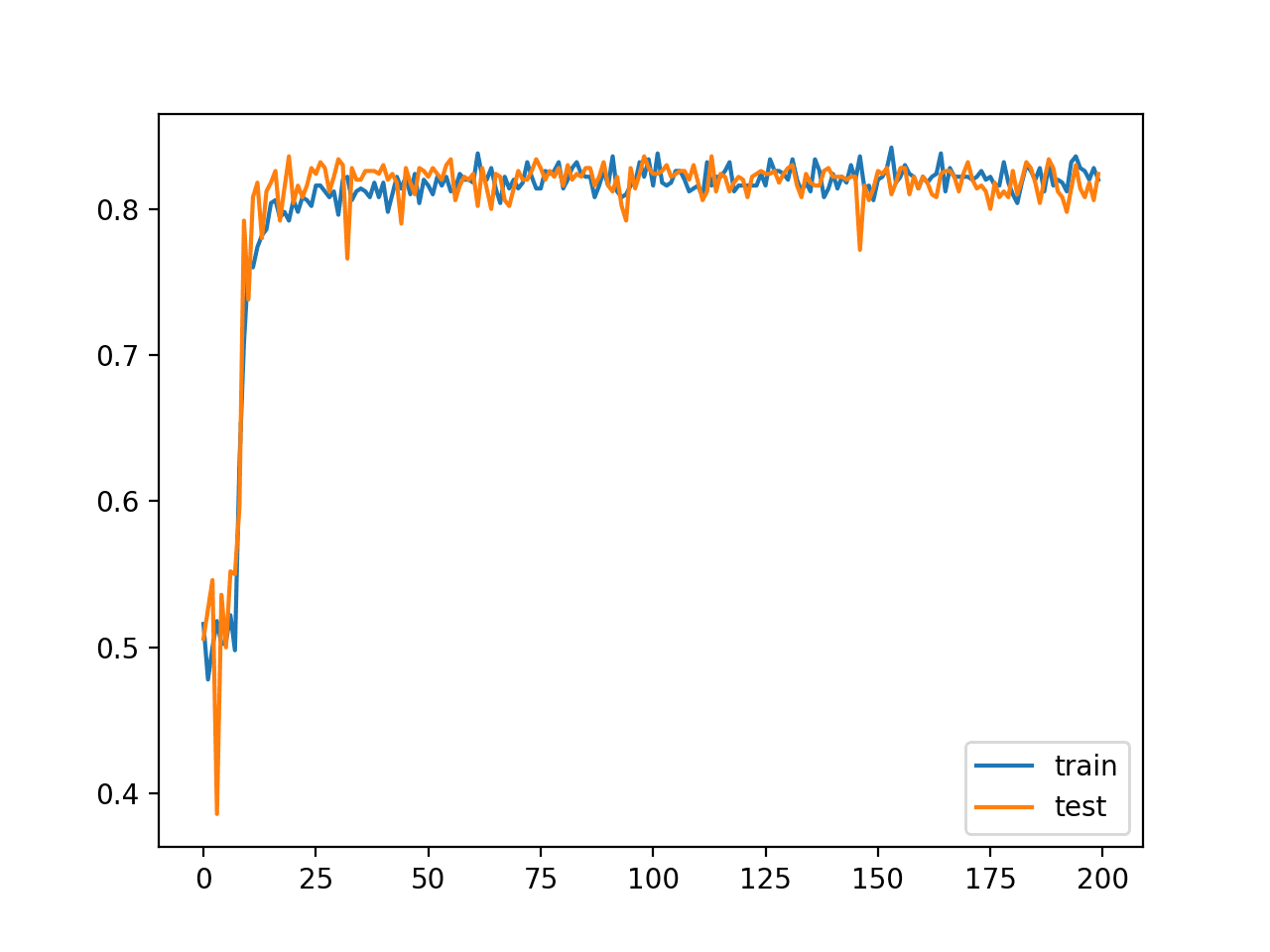
Line Plot of Classification Accuracy on Train and Tests Sets of an MLP Fit With Stochastic Gradient Descent and Smaller Learning Rate
This example highlights the important relationship between batch size and the learning rate. Namely, more noisy updates to the model require a smaller learning rate, whereas less noisy more accurate estimates of the error gradient may be applied to the model more liberally. We can summarize this as follows:
- Batch Gradient Descent: Use a relatively larger learning rate and more training epochs.
- Stochastic Gradient Descent: Use a relatively smaller learning rate and fewer training epochs.
Mini-batch gradient descent provides an alternative approach.
MLP Fit With Minibatch Gradient Descent
An alternative to using stochastic gradient descent and tuning the learning rate is to hold the learning rate constant and to change the batch size.
In effect, it means that we specify the rate of learning or amount of change to apply to the weights each time we estimate the error gradient, but to vary the accuracy of the gradient based on the number of samples used to estimate it.
Holding the learning rate at 0.01 as we did with batch gradient descent, we can set the batch size to 32, a widely adopted default batch size.
# fit model
history = model.fit(trainX, trainy, validation_data=(testX, testy), epochs=200, verbose=0, batch_size=32)
We would expect to get some of the benefits of stochastic gradient descent with a larger learning rate.
The complete example with this modification is listed below.
# mlp for the blobs problem with minibatch gradient descent
from sklearn.datasets.samples_generator import make_blobs
from keras.layers import Dense
from keras.models import Sequential
from keras.optimizers import SGD
from keras.utils import to_categorical
from matplotlib import pyplot
# generate 2d classification dataset
X, y = make_blobs(n_samples=1000, centers=3, n_features=2, cluster_std=2, random_state=2)
# one hot encode output variable
y = to_categorical(y)
# split into train and test
n_train = 500
trainX, testX = X[:n_train, :], X[n_train:, :]
trainy, testy = y[:n_train], y[n_train:]
# define model
model = Sequential()
model.add(Dense(50, input_dim=2, activation='relu', kernel_initializer='he_uniform'))
model.add(Dense(3, activation='softmax'))
# compile model
opt = SGD(lr=0.01, momentum=0.9)
model.compile(loss='categorical_crossentropy', optimizer=opt, metrics=['accuracy'])
# fit model
history = model.fit(trainX, trainy, validation_data=(testX, testy), epochs=200, verbose=0, batch_size=32)
# evaluate the model
_, train_acc = model.evaluate(trainX, trainy, verbose=0)
_, test_acc = model.evaluate(testX, testy, verbose=0)
print('Train: %.3f, Test: %.3f' % (train_acc, test_acc))
# plot training history
pyplot.plot(history.history['acc'], label='train')
pyplot.plot(history.history['val_acc'], label='test')
pyplot.legend()
pyplot.show()
Running the example reports similar performance on both train and test sets, comparable with batch gradient descent and stochastic gradient descent after we reduced the learning rate.
Train: 0.832, Test: 0.812
The line plot shows the dynamics of both stochastic and batch gradient descent. Specifically, the model learns fast and has noisy updates but also stabilizes more towards the end of the run, more so than stochastic gradient descent.
Holding learning rate constant and varying the batch size allows you to dial in the best of both approaches.
Line Plot of Classification Accuracy on Train and Tests Sets of an MLP Fit With Minibatch Gradient Descent
Effect of Batch Size on Model Behavior
We can refit the model with different batch sizes and review the impact the change in batch size has on the speed of learning, stability during learning, and on the final result.
First, we can clean up the code and create a function to prepare the dataset.
# prepare train and test dataset
def prepare_data():
	# generate 2d classification dataset
	X, y = make_blobs(n_samples=1000, centers=3, n_features=2, cluster_std=2, random_state=2)
	# one hot encode output variable
	y = to_categorical(y)
	# split into train and test
	n_train = 500
	trainX, testX = X[:n_train, :], X[n_train:, :]
	trainy, testy = y[:n_train], y[n_train:]
	return trainX, trainy, testX, testy
Next, we can create a function to fit a model on the problem with a given batch size and plot the learning curves of classification accuracy on the train and test datasets.
# fit a model and plot learning curve
def fit_model(trainX, trainy, testX, testy, n_batch):
	# define model
	model = Sequential()
	model.add(Dense(50, input_dim=2, activation='relu', kernel_initializer='he_uniform'))
	model.add(Dense(3, activation='softmax'))
	# compile model
	opt = SGD(lr=0.01, momentum=0.9)
	model.compile(loss='categorical_crossentropy', optimizer=opt, metrics=['accuracy'])
	# fit model
	history = model.fit(trainX, trainy, validation_data=(testX, testy), epochs=200, verbose=0, batch_size=n_batch)
	# plot learning curves
	pyplot.plot(history.history['acc'], label='train')
	pyplot.plot(history.history['val_acc'], label='test')
	pyplot.title('batch='+str(n_batch), pad=-40)
Finally, we can evaluate the model behavior with a suite of different batch sizes while holding everything else about the model constant, including the learning rate.
# prepare dataset
trainX, trainy, testX, testy = prepare_data()
# create learning curves for different batch sizes
batch_sizes = [4, 8, 16, 32, 64, 128, 256, 450]
for i in range(len(batch_sizes)):
	# determine the plot number
	plot_no = 420 + (i+1)
	pyplot.subplot(plot_no)
	# fit model and plot learning curves for a batch size
	fit_model(trainX, trainy, testX, testy, batch_sizes[i])
# show learning curves
pyplot.show()
The result will be a figure with eight plots of model behavior with eight different batch sizes.
Tying this together, the complete example is listed below.
# mlp for the blobs problem with minibatch gradient descent with varied batch size
from sklearn.datasets.samples_generator import make_blobs
from keras.layers import Dense
from keras.models import Sequential
from keras.optimizers import SGD
from keras.utils import to_categorical
from matplotlib import pyplot

# prepare train and test dataset
def prepare_data():
	# generate 2d classification dataset
	X, y = make_blobs(n_samples=1000, centers=3, n_features=2, cluster_std=2, random_state=2)
	# one hot encode output variable
	y = to_categorical(y)
	# split into train and test
	n_train = 500
	trainX, testX = X[:n_train, :], X[n_train:, :]
	trainy, testy = y[:n_train], y[n_train:]
	return trainX, trainy, testX, testy

# fit a model and plot learning curve
def fit_model(trainX, trainy, testX, testy, n_batch):
	# define model
	model = Sequential()
	model.add(Dense(50, input_dim=2, activation='relu', kernel_initializer='he_uniform'))
	model.add(Dense(3, activation='softmax'))
	# compile model
	opt = SGD(lr=0.01, momentum=0.9)
	model.compile(loss='categorical_crossentropy', optimizer=opt, metrics=['accuracy'])
	# fit model
	history = model.fit(trainX, trainy, validation_data=(testX, testy), epochs=200, verbose=0, batch_size=n_batch)
	# plot learning curves
	pyplot.plot(history.history['acc'], label='train')
	pyplot.plot(history.history['val_acc'], label='test')
	pyplot.title('batch='+str(n_batch), pad=-40)

# prepare dataset
trainX, trainy, testX, testy = prepare_data()
# create learning curves for different batch sizes
batch_sizes = [4, 8, 16, 32, 64, 128, 256, 450]
for i in range(len(batch_sizes)):
	# determine the plot number
	plot_no = 420 + (i+1)
	pyplot.subplot(plot_no)
	# fit model and plot learning curves for a batch size
	fit_model(trainX, trainy, testX, testy, batch_sizes[i])
# show learning curves
pyplot.show()
Running the example creates a figure with eight line plots showing the classification accuracy on the train and test sets of models with different batch sizes when using mini-batch gradient descent.
The plots show that small batch results generally in rapid learning but a volatile learning process with higher variance in the classification accuracy. Larger batch sizes slow down the learning process but the final stages result in a convergence to a more stable model exemplified by lower variance in classification accuracy.
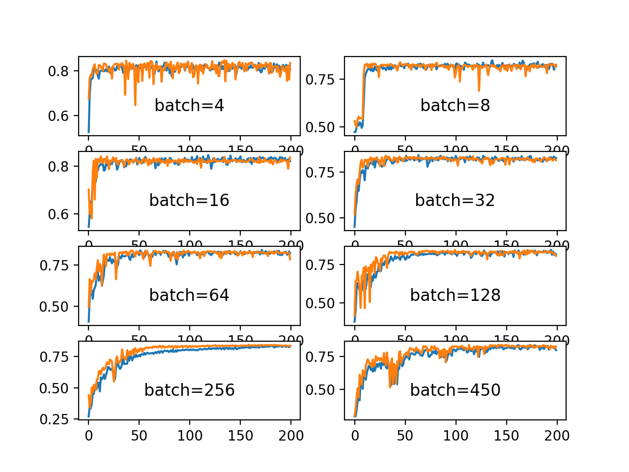
Line Plots of Classification Accuracy on Train and Test Datasets With Different Batch Sizes
Further Reading
This section provides more resources on the topic if you are looking to go deeper.
Posts
Papers
- Revisiting Small Batch Training for Deep Neural Networks, 2018.
- Practical recommendations for gradient-based training of deep architectures, 2012.
Books
- 8.1.3 Batch and Minibatch Algorithms, Deep Learning, 2016.
Articles
Summary
In this tutorial, you discovered three different flavors of gradient descent and how to explore and diagnose the effect of batch size on the learning process.
Specifically, you learned:
- Batch size controls the accuracy of the estimate of the error gradient when training neural networks.
- Batch, Stochastic, and Minibatch gradient descent are the three main flavors of the learning algorithm.
- There is a tension between batch size and the speed and stability of the learning process.
Do you have any questions?
Ask your questions in the comments below and I will do my best to answer.
The post How to Control the Speed and Stability of Training Neural Networks With Gradient Descent Batch Size appeared first on Machine Learning Mastery.