Author: Jason Brownlee
Deep learning neural networks learn how to map inputs to outputs from examples in a training dataset.
The weights of the model are initialized to small random values and updated via an optimization algorithm in response to estimates of error on the training dataset.
Given the use of small weights in the model and the use of error between predictions and expected values, the scale of inputs and outputs used to train the model are an important factor. Unscaled input variables can result in a slow or unstable learning process, whereas unscaled target variables on regression problems can result in exploding gradients causing the learning process to fail.
Data preparation involves using techniques such as the normalization and standardization to rescale input and output variables prior to training a neural network model.
In this tutorial, you will discover how to improve neural network stability and modeling performance by scaling data.
After completing this tutorial, you will know:
- Data scaling is a recommended pre-processing step when working with deep learning neural networks.
- Data scaling can be achieved by normalizing or standardizing real-valued input and output variables.
- How to apply standardization and normalization to improve the performance of a Multilayer Perceptron model on a regression predictive modeling problem.
Let’s get started.

How to Improve Neural Network Stability and Modeling Performance With Data Scaling
Photo by Javier Sanchez Portero, some rights reserved.
Tutorial Overview
This tutorial is divided into six parts; they are:
- The Scale of Your Data Matters
- Data Scaling Methods
- Regression Predictive Modeling Problem
- Multilayer Perceptron With Unscaled Data
- Multilayer Perceptron With Scaled Output Variables
- Multilayer Perceptron With Scaled Input Variables
The Scale of Your Data Matters
Deep learning neural network models learn a mapping from input variables to an output variable.
As such, the scale and distribution of the data drawn from the domain may be different for each variable.
Input variables may have different units (e.g. feet, kilometers, and hours) that, in turn, may mean the variables have different scales.
Differences in the scales across input variables may increase the difficulty of the problem being modeled. An example of this is that large input values (e.g. a spread of hundreds or thousands of units) can result in a model that learns large weight values. A model with large weight values is often unstable, meaning that it may suffer from poor performance during learning and sensitivity to input values resulting in higher generalization error.
One of the most common forms of pre-processing consists of a simple linear rescaling of the input variables.
— Page 298, Neural Networks for Pattern Recognition, 1995.
A target variable with a large spread of values, in turn, may result in large error gradient values causing weight values to change dramatically, making the learning process unstable.
Scaling input and output variables is a critical step in using neural network models.
In practice it is nearly always advantageous to apply pre-processing transformations to the input data before it is presented to a network. Similarly, the outputs of the network are often post-processed to give the required output values.
— Page 296, Neural Networks for Pattern Recognition, 1995.
Scaling Input Variables
The input variables are those that the network takes on the input or visible layer in order to make a prediction.
A good rule of thumb is that input variables should be small values, probably in the range of 0-1 or standardized with a zero mean and a standard deviation of one.
Whether input variables require scaling depends on the specifics of your problem and of each variable.
You may have a sequence of quantities as inputs, such as prices or temperatures.
If the distribution of the quantity is normal, then it should be standardized, otherwise the data should be normalized. This applies if the range of quantity values is large (10s, 100s, etc.) or small (0.01, 0.0001).
If the quantity values are small (near 0-1) and the distribution is limited (e.g. standard deviation near 1) then perhaps you can get away with no scaling of the data.
Problems can be complex and it may not be clear how to best scale input data.
If in doubt, normalize the input sequence. If you have the resources, explore modeling with the raw data, standardized data, and normalized data and see if there is a beneficial difference in the performance of the resulting model.
If the input variables are combined linearly, as in an MLP [Multilayer Perceptron], then it is rarely strictly necessary to standardize the inputs, at least in theory. […] However, there are a variety of practical reasons why standardizing the inputs can make training faster and reduce the chances of getting stuck in local optima.
— Should I normalize/standardize/rescale the data? Neural Nets FAQ
Scaling Output Variables
The output variable is the variable predicted by the network.
You must ensure that the scale of your output variable matches the scale of the activation function (transfer function) on the output layer of your network.
If your output activation function has a range of [0,1], then obviously you must ensure that the target values lie within that range. But it is generally better to choose an output activation function suited to the distribution of the targets than to force your data to conform to the output activation function.
— Should I normalize/standardize/rescale the data? Neural Nets FAQ
If your problem is a regression problem, then the output will be a real value.
This is best modeled with a linear activation function. If the distribution of the value is normal, then you can standardize the output variable. Otherwise, the output variable can be normalized.
Want Better Results with Deep Learning?
Take my free 7-day email crash course now (with sample code).
Click to sign-up and also get a free PDF Ebook version of the course.
Data Scaling Methods
There are two types of scaling of your data that you may want to consider: normalization and standardization.
These can both be achieved using the scikit-learn library.
Data Normalization
Normalization is a rescaling of the data from the original range so that all values are within the range of 0 and 1.
Normalization requires that you know or are able to accurately estimate the minimum and maximum observable values. You may be able to estimate these values from your available data.
A value is normalized as follows:
y = (x - min) / (max - min)
Where the minimum and maximum values pertain to the value x being normalized.
For example, for a dataset, we could guesstimate the min and max observable values as 30 and -10. We can then normalize any value, like 18.8, as follows:
y = (x - min) / (max - min)
y = (18.8 - (-10)) / (30 - (-10))
y = 28.8 / 40
y = 0.72
You can see that if an x value is provided that is outside the bounds of the minimum and maximum values, the resulting value will not be in the range of 0 and 1. You could check for these observations prior to making predictions and either remove them from the dataset or limit them to the pre-defined maximum or minimum values.
You can normalize your dataset using the scikit-learn object MinMaxScaler.
Good practice usage with the MinMaxScaler and other scaling techniques is as follows:
- Fit the scaler using available training data. For normalization, this means the training data will be used to estimate the minimum and maximum observable values. This is done by calling the fit() function.
- Apply the scale to training data. This means you can use the normalized data to train your model. This is done by calling the transform() function.
- Apply the scale to data going forward. This means you can prepare new data in the future on which you want to make predictions.
The default scale for the MinMaxScaler is to rescale variables into the range [0,1], although a preferred scale can be specified via the “feature_range” argument and specify a tuple including the min and the max for all variables.
# create scaler
scaler = MinMaxScaler(feature_range=(-1,1))
If needed, the transform can be inverted. This is useful for converting predictions back into their original scale for reporting or plotting. This can be done by calling the inverse_transform() function.
The example below provides a general demonstration for using the MinMaxScaler to normalize data.
# demonstrate data normalization with sklearn
from sklearn.preprocessing import MinMaxScaler
# load data
data = ...
# create scaler
scaler = MinMaxScaler()
# fit scaler on data
scaler.fit(data)
# apply transform
normalized = scaler.transform(data)
# inverse transform
inverse = scaler.inverse_transform(normalized)
You can also perform the fit and transform in a single step using the fit_transform() function; for example:
# demonstrate data normalization with sklearn
from sklearn.preprocessing import MinMaxScaler
# load data
data = ...
# create scaler
scaler = MinMaxScaler()
# fit and transform in one step
normalized = scaler.fit_transform(data)
# inverse transform
inverse = scaler.inverse_transform(normalized)
Data Standardization
Standardizing a dataset involves rescaling the distribution of values so that the mean of observed values is 0 and the standard deviation is 1. It is sometimes referred to as “whitening.”
This can be thought of as subtracting the mean value or centering the data.
Like normalization, standardization can be useful, and even required in some machine learning algorithms when your data has input values with differing scales.
Standardization assumes that your observations fit a Gaussian distribution (bell curve) with a well behaved mean and standard deviation. You can still standardize your data if this expectation is not met, but you may not get reliable results.
Standardization requires that you know or are able to accurately estimate the mean and standard deviation of observable values. You may be able to estimate these values from your training data.
A value is standardized as follows:
y = (x - mean) / standard_deviation
Where the mean is calculated as:
mean = sum(x) / count(x)
And the standard_deviation is calculated as:
standard_deviation = sqrt( sum( (x - mean)^2 ) / count(x))
We can guesstimate a mean of 10 and a standard deviation of about 5. Using these values, we can standardize the first value of 20.7 as follows:
y = (x - mean) / standard_deviation
y = (20.7 - 10) / 5
y = (10.7) / 5
y = 2.14
The mean and standard deviation estimates of a dataset can be more robust to new data than the minimum and maximum.
You can standardize your dataset using the scikit-learn object StandardScaler.
# demonstrate data standardization with sklearn
from sklearn.preprocessing import StandardScaler
# load data
data = ...
# create scaler
scaler = StandardScaler()
# fit scaler on data
scaler.fit(data)
# apply transform
standardized = scaler.transform(data)
# inverse transform
inverse = scaler.inverse_transform(standardized)
You can also perform the fit and transform in a single step using the fit_transform() function; for example:
# demonstrate data standardization with sklearn
from sklearn.preprocessing import StandardScaler
# load data
data = ...
# create scaler
scaler = StandardScaler()
# fit and transform in one step
standardized = scaler.fit_transform(data)
# inverse transform
inverse = scaler.inverse_transform(standardized)
Regression Predictive Modeling Problem
A regression predictive modeling problem involves predicting a real-valued quantity.
We can use a standard regression problem generator provided by the scikit-learn library in the make_regression() function. This function will generate examples from a simple regression problem with a given number of input variables, statistical noise, and other properties.
We will use this function to define a problem that has 20 input features; 10 of the features will be meaningful and 10 will not be relevant. A total of 1,000 examples will be randomly generated. The pseudorandom number generator will be fixed to ensure that we get the same 1,000 examples each time the code is run.
# generate regression dataset
X, y = make_regression(n_samples=1000, n_features=20, noise=0.1, random_state=1)
Each input variable has a Gaussian distribution, as does the target variable.
We can demonstrate this by creating histograms of some of the input variables and the output variable.
# regression predictive modeling problem
from sklearn.datasets import make_regression
from matplotlib import pyplot
# generate regression dataset
X, y = make_regression(n_samples=1000, n_features=20, noise=0.1, random_state=1)
# histograms of input variables
pyplot.subplot(211)
pyplot.hist(X[:, 0])
pyplot.subplot(212)
pyplot.hist(X[:, 1])
pyplot.show()
# histogram of target variable
pyplot.hist(y)
pyplot.show()
Running the example creates two figures.
The first shows histograms of the first two of the twenty input variables, showing that each has a Gaussian data distribution.
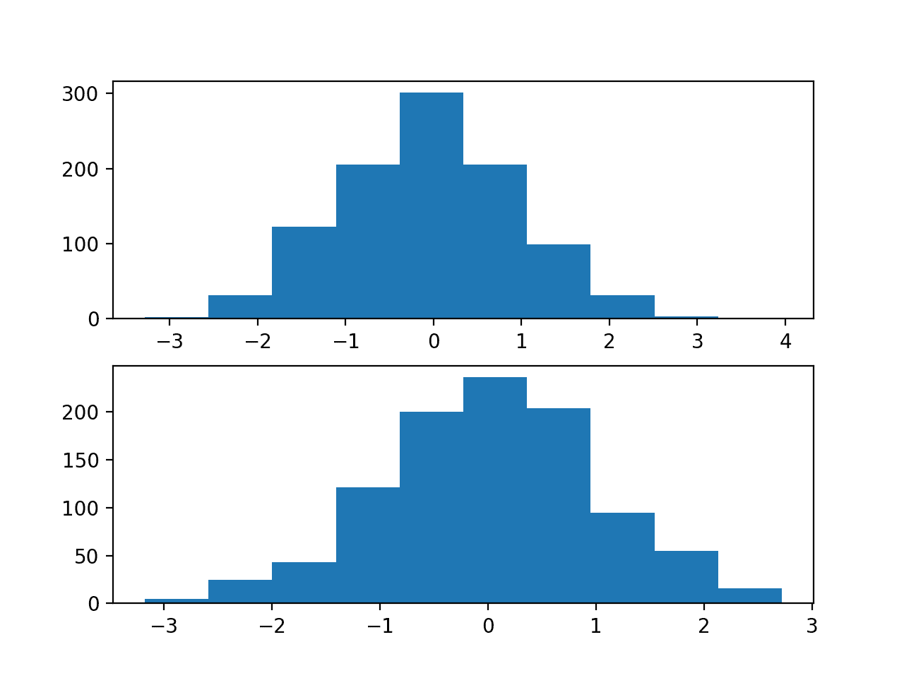
Histograms of Two of the Twenty Input Variables for the Regression Problem
The second figure shows a histogram of the target variable, showing a much larger range for the variable as compared to the input variables and, again, a Gaussian data distribution.
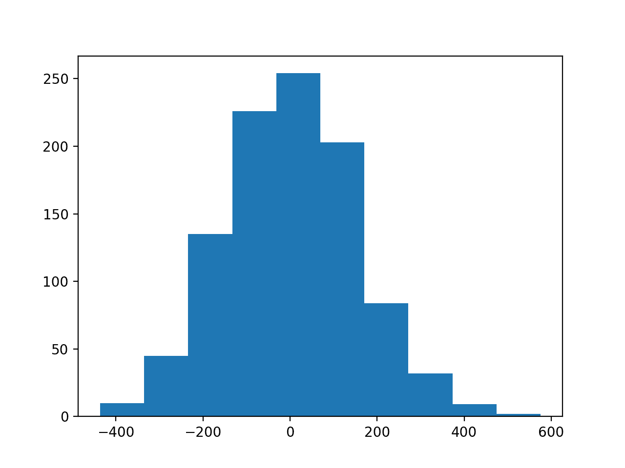
Histogram of the Target Variable for the Regression Problem
Now that we have a regression problem that we can use as the basis for the investigation, we can develop a model to address it.
Multilayer Perceptron With Unscaled Data
We can develop a Multilayer Perceptron (MLP) model for the regression problem.
A model will be demonstrated on the raw data, without any scaling of the input or output variables. We expect that model performance will be generally poor.
The first step is to split the data into train and test sets so that we can fit and evaluate a model. We will generate 1,000 examples from the domain and split the dataset in half, using 500 examples for the train and test datasets.
# split into train and test
n_train = 500
trainX, testX = X[:n_train, :], X[n_train:, :]
trainy, testy = y[:n_train], y[n_train:]
Next, we can define an MLP model. The model will expect 20 inputs in the 20 input variables in the problem.
A single hidden layer will be used with 25 nodes and a rectified linear activation function. The output layer has one node for the single target variable and a linear activation function to predict real values directly.
# define model
model = Sequential()
model.add(Dense(25, input_dim=20, activation='relu', kernel_initializer='he_uniform'))
model.add(Dense(1, activation='linear'))
The mean squared error loss function will be used to optimize the model and the stochastic gradient descent optimization algorithm will be used with the sensible default configuration of a learning rate of 0.01 and a momentum of 0.9.
# compile model
model.compile(loss='mean_squared_error', optimizer=SGD(lr=0.01, momentum=0.9))
The model will be fit for 100 training epochs and the test set will be used as a validation set, evaluated at the end of each training epoch.
The mean squared error is calculated on the train and test datasets at the end of training to get an idea of how well the model learned the problem.
# evaluate the model
train_mse = model.evaluate(trainX, trainy, verbose=0)
test_mse = model.evaluate(testX, testy, verbose=0)
Finally, learning curves of mean squared error on the train and test sets at the end of each training epoch are graphed using line plots, providing learning curves to get an idea of the dynamics of the model while learning the problem.
# plot loss during training
pyplot.title('Mean Squared Error')
pyplot.plot(history.history['loss'], label='train')
pyplot.plot(history.history['val_loss'], label='test')
pyplot.legend()
pyplot.show()
Tying these elements together, the complete example is listed below.
# mlp with unscaled data for the regression problem
from sklearn.datasets import make_regression
from keras.layers import Dense
from keras.models import Sequential
from keras.optimizers import SGD
from matplotlib import pyplot
# generate regression dataset
X, y = make_regression(n_samples=1000, n_features=20, noise=0.1, random_state=1)
# split into train and test
n_train = 500
trainX, testX = X[:n_train, :], X[n_train:, :]
trainy, testy = y[:n_train], y[n_train:]
# define model
model = Sequential()
model.add(Dense(25, input_dim=20, activation='relu', kernel_initializer='he_uniform'))
model.add(Dense(1, activation='linear'))
# compile model
model.compile(loss='mean_squared_error', optimizer=SGD(lr=0.01, momentum=0.9))
# fit model
history = model.fit(trainX, trainy, validation_data=(testX, testy), epochs=100, verbose=0)
# evaluate the model
train_mse = model.evaluate(trainX, trainy, verbose=0)
test_mse = model.evaluate(testX, testy, verbose=0)
print('Train: %.3f, Test: %.3f' % (train_mse, test_mse))
# plot loss during training
pyplot.title('Mean Squared Error')
pyplot.plot(history.history['loss'], label='train')
pyplot.plot(history.history['val_loss'], label='test')
pyplot.legend()
pyplot.show()
Running the example fits the model and calculates the mean squared error on the train and test sets.
In this case, the model is unable to learn the problem, resulting in predictions of NaN values. The model weights exploded during training given the very large errors and, in turn, error gradients calculated for weight updates.
Train: nan, Test: nan
This demonstrates that, at the very least, some data scaling is required for the target variable.
A line plot of training history is created but does not show anything as the model almost immediately results in a NaN mean squared error.
Multilayer Perceptron With Scaled Output Variables
The MLP model can be updated to scale the target variable.
Reducing the scale of the target variable will, in turn, reduce the size of the gradient used to update the weights and result in a more stable model and training process.
Given the Gaussian distribution of the target variable, a natural method for rescaling the variable would be to standardize the variable. This requires estimating the mean and standard deviation of the variable and using these estimates to perform the rescaling.
It is best practice is to estimate the mean and standard deviation of the training dataset and use these variables to scale the train and test dataset. This is to avoid any data leakage during the model evaluation process.
The scikit-learn transformers expect input data to be matrices of rows and columns, therefore the 1D arrays for the target variable will have to be reshaped into 2D arrays prior to the transforms.
# reshape 1d arrays to 2d arrays
trainy = trainy.reshape(len(trainy), 1)
testy = testy.reshape(len(trainy), 1)
We can then create and apply the StandardScaler to rescale the target variable.
# created scaler
scaler = StandardScaler()
# fit scaler on training dataset
scaler.fit(trainy)
# transform training dataset
trainy = scaler.transform(trainy)
# transform test dataset
testy = scaler.transform(testy)
Rescaling the target variable means that estimating the performance of the model and plotting the learning curves will calculate an MSE in squared units of the scaled variable rather than squared units of the original scale. This can make interpreting the error within the context of the domain challenging.
In practice, it may be helpful to estimate the performance of the model by first inverting the transform on the test dataset target variable and on the model predictions and estimating model performance using the root mean squared error on the unscaled data. This is left as an exercise to the reader.
The complete example of standardizing the target variable for the MLP on the regression problem is listed below.
# mlp with scaled outputs on the regression problem
from sklearn.datasets import make_regression
from sklearn.preprocessing import StandardScaler
from keras.layers import Dense
from keras.models import Sequential
from keras.optimizers import SGD
from matplotlib import pyplot
# generate regression dataset
X, y = make_regression(n_samples=1000, n_features=20, noise=0.1, random_state=1)
# split into train and test
n_train = 500
trainX, testX = X[:n_train, :], X[n_train:, :]
trainy, testy = y[:n_train], y[n_train:]
# reshape 1d arrays to 2d arrays
trainy = trainy.reshape(len(trainy), 1)
testy = testy.reshape(len(trainy), 1)
# created scaler
scaler = StandardScaler()
# fit scaler on training dataset
scaler.fit(trainy)
# transform training dataset
trainy = scaler.transform(trainy)
# transform test dataset
testy = scaler.transform(testy)
# define model
model = Sequential()
model.add(Dense(25, input_dim=20, activation='relu', kernel_initializer='he_uniform'))
model.add(Dense(1, activation='linear'))
# compile model
model.compile(loss='mean_squared_error', optimizer=SGD(lr=0.01, momentum=0.9))
# fit model
history = model.fit(trainX, trainy, validation_data=(testX, testy), epochs=100, verbose=0)
# evaluate the model
train_mse = model.evaluate(trainX, trainy, verbose=0)
test_mse = model.evaluate(testX, testy, verbose=0)
print('Train: %.3f, Test: %.3f' % (train_mse, test_mse))
# plot loss during training
pyplot.title('Loss / Mean Squared Error')
pyplot.plot(history.history['loss'], label='train')
pyplot.plot(history.history['val_loss'], label='test')
pyplot.legend()
pyplot.show()
Running the example fits the model and calculates the mean squared error on the train and test sets.
Your specific results may vary given the stochastic nature of the learning algorithm. Try running the example a few times.
In this case, the model does appear to learn the problem and achieves near-zero mean squared error, at least to three decimal places.
Train: 0.003, Test: 0.007
A line plot of the mean squared error on the train (blue) and test (orange) dataset over each training epoch is created.
In this case, we can see that the model rapidly learns to effectively map inputs to outputs for the regression problem and achieves good performance on both datasets over the course of the run, neither overfitting or underfitting the training dataset.
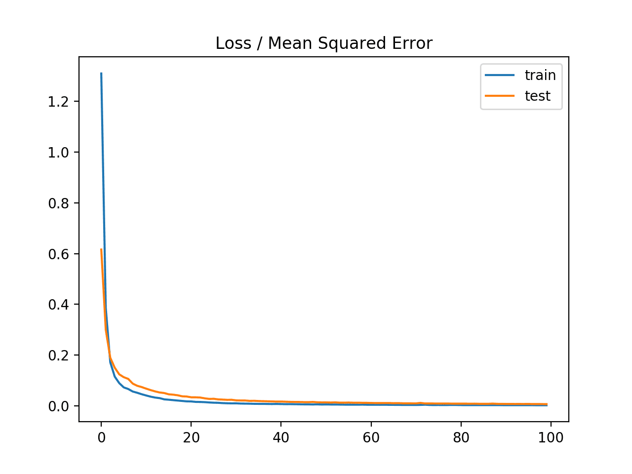
Line Plot of Mean Squared Error on the Train a Test Datasets for Each Training Epoch
It may be interesting to repeat this experiment and normalize the target variable instead and compare results.
Multilayer Perceptron With Scaled Input Variables
We have seen that data scaling can stabilize the training process when fitting a model for regression with a target variable that has a wide spread.
It is also possible to improve the stability and performance of the model by scaling the input variables.
In this section, we will design an experiment to compare the performance of different scaling methods for the input variables.
The input variables also have a Gaussian data distribution, like the target variable, therefore we would expect that standardizing the data would be the best approach. This is not always the case.
We can compare the performance of the unscaled input variables to models fit with either standardized and normalized input variables.
The first step is to define a function to create the same 1,000 data samples, split them into train and test sets, and apply the data scaling methods specified via input arguments. The get_dataset() function below implements this, requiring the scaler to be provided for the input and target variables and returns the train and test datasets split into input and output components ready to train and evaluate a model.
# prepare dataset with input and output scalers, can be none
def get_dataset(input_scaler, output_scaler):
	# generate dataset
	X, y = make_regression(n_samples=1000, n_features=20, noise=0.1, random_state=1)
	# split into train and test
	n_train = 500
	trainX, testX = X[:n_train, :], X[n_train:, :]
	trainy, testy = y[:n_train], y[n_train:]
	# scale inputs
	if input_scaler is not None:
		# fit scaler
		input_scaler.fit(trainX)
		# transform training dataset
		trainX = input_scaler.transform(trainX)
		# transform test dataset
		testX = input_scaler.transform(testX)
	if output_scaler is not None:
		# reshape 1d arrays to 2d arrays
		trainy = trainy.reshape(len(trainy), 1)
		testy = testy.reshape(len(trainy), 1)
		# fit scaler on training dataset
		output_scaler.fit(trainy)
		# transform training dataset
		trainy = output_scaler.transform(trainy)
		# transform test dataset
		testy = output_scaler.transform(testy)
	return trainX, trainy, testX, testy
Next, we can define a function to fit an MLP model on a given dataset and return the mean squared error for the fit model on the test dataset.
The evaluate_model() function below implements this behavior.
# fit and evaluate mse of model on test set
def evaluate_model(trainX, trainy, testX, testy):
	# define model
	model = Sequential()
	model.add(Dense(25, input_dim=20, activation='relu', kernel_initializer='he_uniform'))
	model.add(Dense(1, activation='linear'))
	# compile model
	model.compile(loss='mean_squared_error', optimizer=SGD(lr=0.01, momentum=0.9))
	# fit model
	model.fit(trainX, trainy, epochs=100, verbose=0)
	# evaluate the model
	test_mse = model.evaluate(testX, testy, verbose=0)
	return test_mse
Neural networks are trained using a stochastic learning algorithm. This means that the same model fit on the same data may result in a different performance.
We can address this in our experiment by repeating the evaluation of each model configuration, in this case a choice of data scaling, multiple times and report performance as the mean of the error scores across all of the runs. We will repeat each run 30 times to ensure the mean is statistically robust.
The repeated_evaluation() function below implements this, taking the scaler for input and output variables as arguments, evaluating a model 30 times with those scalers, printing error scores along the way, and returning a list of the calculated error scores from each run.
# evaluate model multiple times with given input and output scalers
def repeated_evaluation(input_scaler, output_scaler, n_repeats=30):
	# get dataset
	trainX, trainy, testX, testy = get_dataset(input_scaler, output_scaler)
	# repeated evaluation of model
	results = list()
	for _ in range(n_repeats):
		test_mse = evaluate_model(trainX, trainy, testX, testy)
		print('>%.3f' % test_mse)
		results.append(test_mse)
	return results
Finally, we can run the experiment and evaluate the same model on the same dataset three different ways:
- No scaling of inputs, standardized outputs.
- Normalized inputs, standardized outputs.
- Standardized inputs, standardized outputs.
The mean and standard deviation of the error for each configuration is reported, then box and whisker plots are created to summarize the error scores for each configuration.
# unscaled inputs
results_unscaled_inputs = repeated_evaluation(None, StandardScaler())
# normalized inputs
results_normalized_inputs = repeated_evaluation(MinMaxScaler(), StandardScaler())
# standardized inputs
results_standardized_inputs = repeated_evaluation(StandardScaler(), StandardScaler())
# summarize results
print('Unscaled: %.3f (%.3f)' % (mean(results_unscaled_inputs), std(results_unscaled_inputs)))
print('Normalized: %.3f (%.3f)' % (mean(results_normalized_inputs), std(results_normalized_inputs)))
print('Standardized: %.3f (%.3f)' % (mean(results_standardized_inputs), std(results_standardized_inputs)))
# plot results
results = [results_unscaled_inputs, results_normalized_inputs, results_standardized_inputs]
labels = ['unscaled', 'normalized', 'standardized']
pyplot.boxplot(results, labels=labels)
pyplot.show()
Tying these elements together, the complete example is listed below.
# compare scaling methods for mlp inputs on regression problem
from sklearn.datasets import make_regression
from sklearn.preprocessing import StandardScaler
from sklearn.preprocessing import MinMaxScaler
from keras.layers import Dense
from keras.models import Sequential
from keras.optimizers import SGD
from matplotlib import pyplot
from numpy import mean
from numpy import std

# prepare dataset with input and output scalers, can be none
def get_dataset(input_scaler, output_scaler):
	# generate dataset
	X, y = make_regression(n_samples=1000, n_features=20, noise=0.1, random_state=1)
	# split into train and test
	n_train = 500
	trainX, testX = X[:n_train, :], X[n_train:, :]
	trainy, testy = y[:n_train], y[n_train:]
	# scale inputs
	if input_scaler is not None:
		# fit scaler
		input_scaler.fit(trainX)
		# transform training dataset
		trainX = input_scaler.transform(trainX)
		# transform test dataset
		testX = input_scaler.transform(testX)
	if output_scaler is not None:
		# reshape 1d arrays to 2d arrays
		trainy = trainy.reshape(len(trainy), 1)
		testy = testy.reshape(len(trainy), 1)
		# fit scaler on training dataset
		output_scaler.fit(trainy)
		# transform training dataset
		trainy = output_scaler.transform(trainy)
		# transform test dataset
		testy = output_scaler.transform(testy)
	return trainX, trainy, testX, testy

# fit and evaluate mse of model on test set
def evaluate_model(trainX, trainy, testX, testy):
	# define model
	model = Sequential()
	model.add(Dense(25, input_dim=20, activation='relu', kernel_initializer='he_uniform'))
	model.add(Dense(1, activation='linear'))
	# compile model
	model.compile(loss='mean_squared_error', optimizer=SGD(lr=0.01, momentum=0.9))
	# fit model
	model.fit(trainX, trainy, epochs=100, verbose=0)
	# evaluate the model
	test_mse = model.evaluate(testX, testy, verbose=0)
	return test_mse

# evaluate model multiple times with given input and output scalers
def repeated_evaluation(input_scaler, output_scaler, n_repeats=30):
	# get dataset
	trainX, trainy, testX, testy = get_dataset(input_scaler, output_scaler)
	# repeated evaluation of model
	results = list()
	for _ in range(n_repeats):
		test_mse = evaluate_model(trainX, trainy, testX, testy)
		print('>%.3f' % test_mse)
		results.append(test_mse)
	return results

# unscaled inputs
results_unscaled_inputs = repeated_evaluation(None, StandardScaler())
# normalized inputs
results_normalized_inputs = repeated_evaluation(MinMaxScaler(), StandardScaler())
# standardized inputs
results_standardized_inputs = repeated_evaluation(StandardScaler(), StandardScaler())
# summarize results
print('Unscaled: %.3f (%.3f)' % (mean(results_unscaled_inputs), std(results_unscaled_inputs)))
print('Normalized: %.3f (%.3f)' % (mean(results_normalized_inputs), std(results_normalized_inputs)))
print('Standardized: %.3f (%.3f)' % (mean(results_standardized_inputs), std(results_standardized_inputs)))
# plot results
results = [results_unscaled_inputs, results_normalized_inputs, results_standardized_inputs]
labels = ['unscaled', 'normalized', 'standardized']
pyplot.boxplot(results, labels=labels)
pyplot.show()
Running the example prints the mean squared error for each model run along the way.
After each of the three configurations have been evaluated 30 times each, the mean errors for each are reported.
Your specific results may vary, but the general trend should be the same as is listed below.
In this case, we can see that as we expected, scaling the input variables does result in a model with better performance. Unexpectedly, better performance is seen using normalized inputs instead of standardized inputs. This may be related to the choice of the rectified linear activation function in the first hidden layer.
...
>0.010
>0.012
>0.005
>0.008
>0.008
Unscaled: 0.007 (0.004)
Normalized: 0.001 (0.000)
Standardized: 0.008 (0.004)
A figure with three box and whisker plots is created summarizing the spread of error scores for each configuration.
The plots show that there was little difference between the distributions of error scores for the unscaled and standardized input variables, and that the normalized input variables result in better performance and more stable or a tighter distribution of error scores.
These results highlight that it is important to actually experiment and confirm the results of data scaling methods rather than assuming that a given data preparation scheme will work best based on the observed distribution of the data.
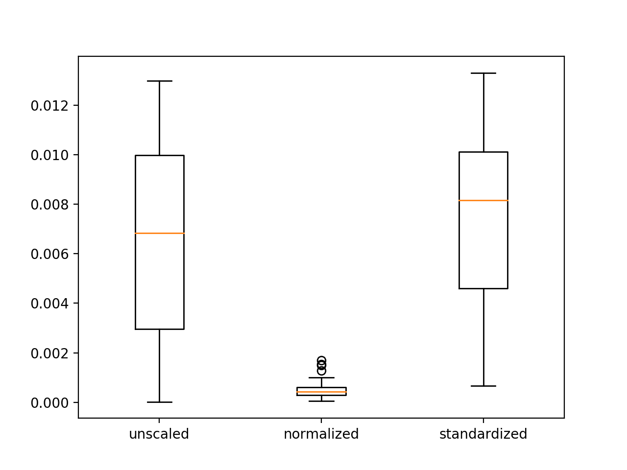
Box and Whisker Plots of Mean Squared Error With Unscaled, Normalized and Standardized Input Variables for the Regression Problem
Extensions
This section lists some ideas for extending the tutorial that you may wish to explore.
- Normalize Target Variable. Update the example and normalize instead of standardize the target variable and compare results.
- Compared Scaling for Target Variable. Update the example to compare standardizing and normalizing the target variable using repeated experiments and compare the results.
- Other Scales. Update the example to evaluate other min/max scales when normalizing and compare performance, e.g. [-1, 1] and [0.0, 0.5].
If you explore any of these extensions, I’d love to know.
Further Reading
This section provides more resources on the topic if you are looking to go deeper.
Posts
- How to Scale Data for Long Short-Term Memory Networks in Python
- How to Scale Machine Learning Data From Scratch With Python
- How to Normalize and Standardize Time Series Data in Python
- How to Prepare Your Data for Machine Learning in Python with Scikit-Learn
Books
- Section 8.2 Input normalization and encoding, Neural Networks for Pattern Recognition, 1995.
API
- sklearn.datasets.make_regression API
- sklearn.preprocessing.MinMaxScaler API
- sklearn.preprocessing.StandardScaler API
Articles
Summary
In this tutorial, you discovered how to improve neural network stability and modeling performance by scaling data.
Specifically, you learned:
- Data scaling is a recommended pre-processing step when working with deep learning neural networks.
- Data scaling can be achieved by normalizing or standardizing real-valued input and output variables.
- How to apply standardization and normalization to improve the performance of a Multilayer Perceptron model on a regression predictive modeling problem.
Do you have any questions?
Ask your questions in the comments below and I will do my best to answer.
The post How to Improve Neural Network Stability and Modeling Performance With Data Scaling appeared first on Machine Learning Mastery.