
Author: Jason Brownlee
It can be convenient to use a standard computer vision dataset when getting started with deep learning methods for computer vision.
Standard datasets are often well understood, small, and easy to load. They can provide the basis for testing techniques and reproducing results in order to build confidence with libraries and methods.
In this tutorial, you will discover the standard computer vision datasets provided with the Keras deep learning library.
After completing this tutorial, you will know:
- The API and idioms for downloading standard computer vision datasets using Keras.
- The structure, nature, and top results for the MNIST, Fashion-MNIST, CIFAR-10, and CIFAR-100 computer vision datasets.
- How to load and visualize standard computer vision datasets using the Keras API.
Let’s get started.
How to Load and Visualize Standard Computer Vision Datasets With Keras
Photo by Marina del Castell, some rights reserved.
Tutorial Overview
This tutorial is divided into five parts; they are:
- Keras Computer Vision Datasets
- MNIST Dataset
- Fashion-MNIST Dataset
- CIFAR-10 Dataset
- CIFAR-100 Dataset
Keras Computer Vision Datasets
The Keras deep learning library provides access to four standard computer vision datasets.
This is particularly helpful as it allows you to rapidly start testing model architectures and configurations for computer vision.
Four specific multi-class image classification dataset are provided; they are:
- MNIST: Classify photos of handwritten digits (10 classes).
- Fashion-MNIST: Classify photos of items of clothing (10 classes).
- CIFAR-10: Classify small photos of objects (10 classes).
- CIFAR-100: Classify small photos of common objects (100 classes).
The datasets are available under the keras.datasets module via dataset-specific load functions.
After a call to the load function, the dataset is downloaded to your workstation and stored in the ~/.keras directory under a “datasets” subdirectory. The datasets are stored in a compressed format, but may also include additional metadata.
After the first call to a dataset-specific load function and the dataset is downloaded, the dataset does not need to be downloaded again. Subsequent calls will load the dataset immediately from disk.
The load functions return two tuples, the first containing the input and output elements for samples in the training dataset, and the second containing the input and output elements for samples in the test dataset. The splits between train and test datasets often follow a standard split, used when benchmarking algorithms on the dataset.
The standard idiom for loading the datasets is as follows:
...
# load dataset
(trainX, trainy), (testX, testy) = load_data()
Each of the train and test X and y elements are NumPy arrays of pixel or class values respectively.
Two of the datasets contain grayscale images and two contain color images. The shape of the grayscale images must be converted from two-dimensional to three-dimensional arrays to match the preferred channel ordering of Keras. For example:
# reshape grayscale images to have a single channel
width, height, channels = trainX.shape[1], trainX.shape[2], 1
trainX = trainX.reshape((trainX.shape[0], width, height, channels))
testX = testX.reshape((testX.shape[0], width, height, channels))
Both grayscale and color image pixel data are stored as unsigned integer values with values between 0 and 255.
Before modeling, the image data will need to be rescaled, e.g. such as normalization to the range 0-1 and perhaps further standardized. For example:
# normalize pixel values
trainX = trainX.astype('float32') / 255
testX = testX.astype('float32') / 255
The output elements of each sample (y) are stored as class integer values. Each problem is a multi-class classification problem (more than two classes); as such, it is common practice to one hot encode the class values prior to modeling. This can be achieved using the to_categorical() function provided by Keras; for example:
...
# one hot encode target values
trainy = to_categorical(trainy)
testy = to_categorical(testy)
Now that we are familiar with the idioms for working with the standard computer vision datasets provided by Keras, let’s take a closer look at each dataset in turn.
Note, the examples in this tutorial assume that you have internet access and may download the datasets the first time each example is run on your system. The download speed will depend on the speed of your internet connection and you are recommended to run the examples from the command line.
Want Results with Deep Learning for Computer Vision?
Take my free 7-day email crash course now (with sample code).
Click to sign-up and also get a free PDF Ebook version of the course.
MNIST Dataset
The MNIST dataset is an acronym that stands for the Modified National Institute of Standards and Technology dataset.
It is a dataset of 60,000 small square 28×28 pixel grayscale images of handwritten single digits between 0 and 9.
The task is to classify a given image of a handwritten digit into one of 10 classes representing integer values from 0 to 9, inclusively.
It is a widely used and deeply understood dataset, and for the most part, is “solved.” Top-performing models are deep learning convolutional neural networks that achieve a classification accuracy of above 99%, with an error rate between 0.4 %and 0.2% on the holdout test dataset.
The example below loads the MNIST dataset using the Keras API and creates a plot of the first 9 images in the training dataset.
# example of loading the mnist dataset
from keras.datasets import mnist
from matplotlib import pyplot
# load dataset
(trainX, trainy), (testX, testy) = mnist.load_data()
# summarize loaded dataset
print('Train: X=%s, y=%s' % (trainX.shape, trainy.shape))
print('Test: X=%s, y=%s' % (testX.shape, testy.shape))
# plot first few images
for i in range(9):
	# define subplot
	pyplot.subplot(330 + 1 + i)
	# plot raw pixel data
	pyplot.imshow(trainX[i], cmap=pyplot.get_cmap('gray'))
# show the figure
pyplot.show()
Running the example loads the MNIST train and test dataset and prints their shape.
We can see that there are 60,000 examples in the training dataset and 10,000 in the test dataset and that images are indeed square with 28×28 pixels.
Train: X=(60000, 28, 28), y=(60000,)
Test: X=(10000, 28, 28), y=(10000,)
A plot of the first nine images in the dataset is also created showing the natural handwritten nature of the images to be classified.
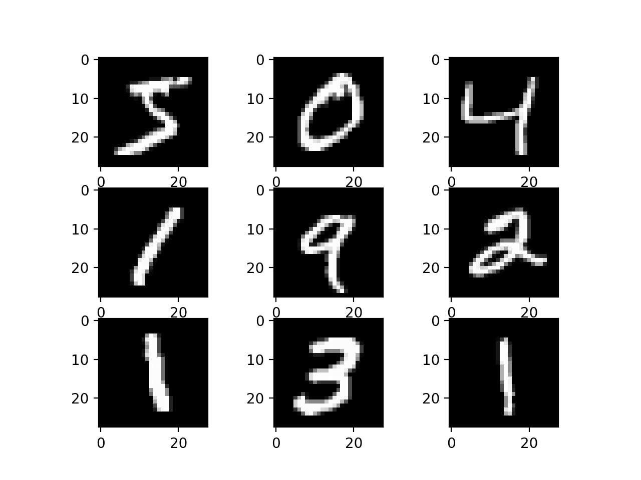
Plot of a Subset of Images From the MNIST Dataset
Fashion-MNIST Dataset
The Fashion-MNIST is proposed as a more challenging replacement dataset for the MNIST dataset.
It is a dataset comprised of 60,000 small square 28×28 pixel grayscale images of items of 10 types of clothing, such as shoes, t-shirts, dresses, and more.
It is a more challenging classification problem than MNIST and top results are achieved by deep learning convolutional networks with a classification accuracy of about 95% to 96% on the holdout test dataset.
The example below loads the Fashion-MNIST dataset using the Keras API and creates a plot of the first nine images in the training dataset.
# example of loading the fashion mnist dataset
from matplotlib import pyplot
from keras.datasets import fashion_mnist
# load dataset
(trainX, trainy), (testX, testy) = fashion_mnist.load_data()
# summarize loaded dataset
print('Train: X=%s, y=%s' % (trainX.shape, trainy.shape))
print('Test: X=%s, y=%s' % (testX.shape, testy.shape))
# plot first few images
for i in range(9):
	# define subplot
	pyplot.subplot(330 + 1 + i)
	# plot raw pixel data
	pyplot.imshow(trainX[i], cmap=pyplot.get_cmap('gray'))
# show the figure
pyplot.show()
Running the example loads the Fashion-MNIST train and test dataset and prints their shape.
We can see that there are 60,000 examples in the training dataset and 10,000 in the test dataset and that images are indeed square with 28×28 pixels.
Train: X=(60000, 28, 28), y=(60000,)
Test: X=(10000, 28, 28), y=(10000,)
A plot of the first nine images in the dataset is also created, showing that indeed the images are grayscale photographs of items of clothing.
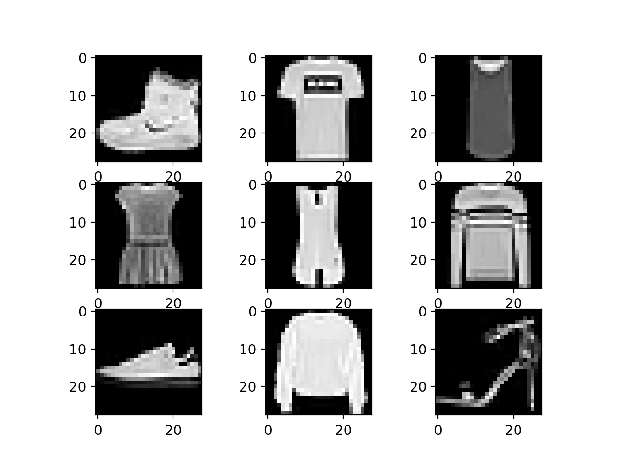
Plot of a Subset of Images From the Fashion-MNIST Dataset
CIFAR-10 Dataset
CIFAR is an acronym that stands for the Canadian Institute For Advanced Research and the CIFAR-10 dataset was developed along with the CIFAR-100 dataset (covered in the next section) by researchers at the CIFAR institute.
The dataset is comprised of 60,000 32×32 pixel color photographs of objects from 10 classes, such as frogs, birds, cats, ships, etc.
These are very small images, much smaller than a typical photograph, and the dataset is intended for computer vision research.
CIFAR-10 is a dataset and was widely used for benchmarking computer vision algorithms in the field of machine learning. The problem is “solved.” Top performance on the problem is achieved by deep learning convolutional neural networks with a classification accuracy above 96% or 97% on the test dataset.
The example below loads the CIFAR-10 dataset using the Keras API and creates a plot of the first nine images in the training dataset.
# example of loading the cifar10 dataset
from matplotlib import pyplot
from keras.datasets import cifar10
# load dataset
(trainX, trainy), (testX, testy) = cifar10.load_data()
# summarize loaded dataset
print('Train: X=%s, y=%s' % (trainX.shape, trainy.shape))
print('Test: X=%s, y=%s' % (testX.shape, testy.shape))
# plot first few images
for i in range(9):
	# define subplot
	pyplot.subplot(330 + 1 + i)
	# plot raw pixel data
	pyplot.imshow(trainX[i])
# show the figure
pyplot.show()
Running the example loads the CIFAR-10 train and test dataset and prints their shape.
We can see that there are 50,000 examples in the training dataset and 10,000 in the test dataset and that images are indeed square with 32×32 pixels and color, with three channels.
Train: X=(50000, 32, 32, 3), y=(50000, 1)
Test: X=(10000, 32, 32, 3), y=(10000, 1)
A plot of the first nine images in the dataset is also created. It is clear that the images are indeed very small compared to modern photographs; it can be challenging to see what exactly is represented in some of the images given the extremely low resolution.
This low resolution is likely the cause of the limited performance that top-of-the-line algorithms are able to achieve on the dataset.
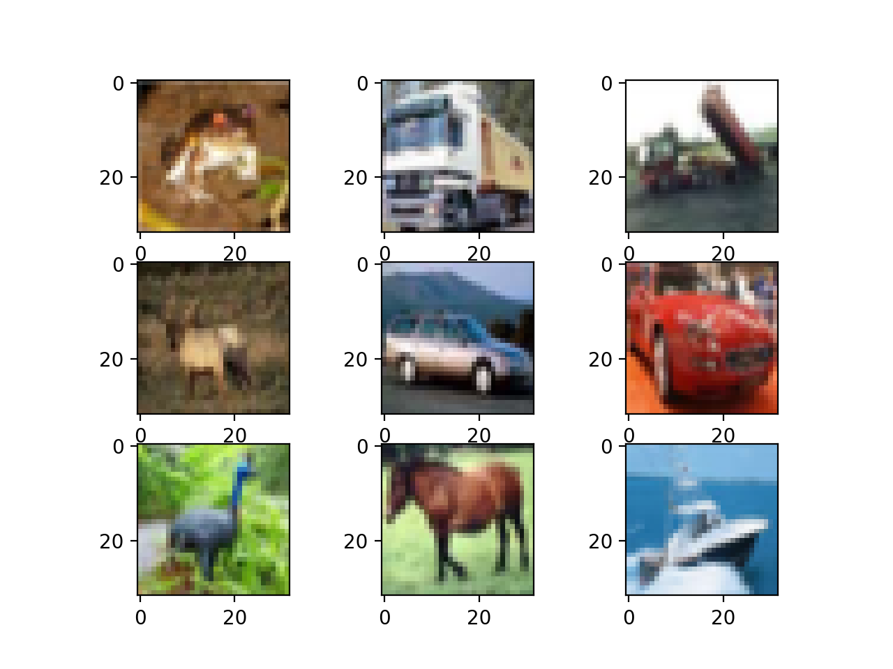
Plot of a Subset of Images From the CIFAR-10 Dataset
CIFAR-100 Dataset
The CIFAR-100 dataset was prepared along with the CIFAR-10 dataset by academics at the Canadian Institute For Advanced Research (CIFAR).
The dataset is comprised of 60,000 32×32 pixel color photographs of objects from 100 classes, such as fish, flowers, insects, and much more.
Like CIFAR-10, the images are intentionally small and unrealistic photographs and the dataset is intended for computer vision research.
The example below loads the CIFAR-100 dataset using the Keras API and creates a plot of the first nine images in the training dataset.
# example of loading the cifar100 dataset
from matplotlib import pyplot
from keras.datasets import cifar100
# load dataset
(trainX, trainy), (testX, testy) = cifar100.load_data()
# summarize loaded dataset
print('Train: X=%s, y=%s' % (trainX.shape, trainy.shape))
print('Test: X=%s, y=%s' % (testX.shape, testy.shape))
# plot first few images
for i in range(9):
	# define subplot
	pyplot.subplot(330 + 1 + i)
	# plot raw pixel data
	pyplot.imshow(trainX[i])
# show the figure
pyplot.show()
Running the example loads the CIFAR-100 train and test dataset and prints their shape.
We can see that there are 50,000 examples in the training dataset and 10,000 in the test dataset and that images are indeed square with 32×32 pixels and color, with three channels.
Train: X=(50000, 32, 32, 3), y=(50000, 1)
Test: X=(10000, 32, 32, 3), y=(10000, 1)
A plot of the first nine images in the dataset is also created, and like CIFAR-10, the low resolution of the images can make it challenging to clearly see what is present in some photos.
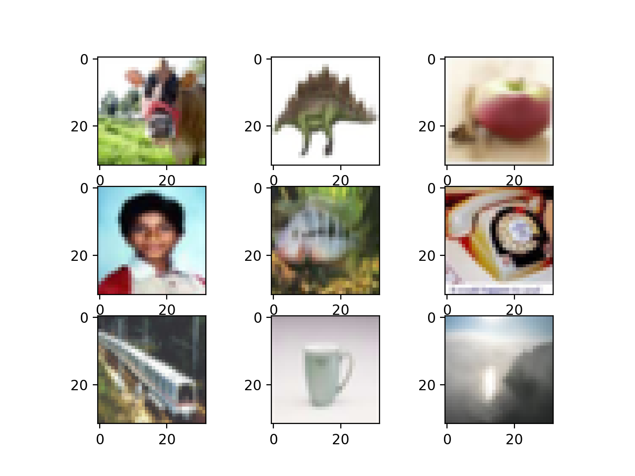
Plot of a Subset of Images From the CIFAR-100 Dataset
Although there are images organized into 100 classes, the 100 classes are organized into 20 super-classes, e.g. groups of common classes.
Keras will return labels for 100 classes by default, although labels can be retrieved by setting the “label_mode” argument to “coarse” (instead of the default “fine“) when calling the load_data() function. For example:
# load coarse labels
(trainX, trainy), (testX, testy) = cifar100.load_data(label_mode='coarse')
The difference is made clear when the labels are one hot encoded using the to_categorical() function, where instead of each output vector having 100 dimensions, it will only have 20. The example below demonstrates this by loading the dataset with course labels and encoding the class labels.
# example of loading the cifar100 dataset with coarse labels
from keras.datasets import cifar100
from keras.utils import to_categorical
# load coarse labels
(trainX, trainy), (testX, testy) = cifar100.load_data(label_mode='coarse')
# one hot encode target values
trainy = to_categorical(trainy)
testy = to_categorical(testy)
# summarize loaded dataset
print('Train: X=%s, y=%s' % (trainX.shape, trainy.shape))
print('Test: X=%s, y=%s' % (testX.shape, testy.shape))
Running the example loads the CIFAR-100 dataset as before, but images are now classified as belonging to one of the twenty super-classes.
The class labels are one hot encoded and we can see that each label is represented by a twenty element vector instead of a 100 element vector we would expect for the fine class labels.
Train: X=(50000, 32, 32, 3), y=(50000, 20)
Test: X=(10000, 32, 32, 3), y=(10000, 20)
Further Reading
This section provides more resources on the topic if you are looking to go deeper.
APIs
Articles
- MNIST database, Wikipedia.
- Classification datasets results, What is the class of this image?
- Fashion-MNIST GitHub Repository
- CIFAR-10, Wikipedia.
- The CIFAR-10 dataset and CIFAR-100 datasets.
Summary
In this tutorial, you discovered the standard computer vision datasets provided with the Keras deep learning library.
Specifically, you learned:
- The API and idioms for downloading standard computer vision datasets using Keras.
- The structure, nature, and top results for the MNIST, Fashion-MNIST, CIFAR-10 and CIFAR-100 computer vision datasets.
- How to load and visualize standard computer vision datasets using the Keras API.
Do you have any questions?
Ask your questions in the comments below and I will do my best to answer.
The post How to Load and Visualize Standard Computer Vision Datasets With Keras appeared first on Machine Learning Mastery.