
Author: Jason Brownlee
Deep Learning for Computer Vision Crash Course.
Bring Deep Learning Methods to Your Computer Vision Project in 7 Days.
We are awash in digital images from photos, videos, Instagram, YouTube, and increasingly live video streams.
Working with image data is hard as it requires drawing upon knowledge from diverse domains such as digital signal processing, machine learning, statistical methods, and these days, deep learning.
Deep learning methods are out-competing the classical and statistical methods on some challenging computer vision problems with singular and simpler models.
In this crash course, you will discover how you can get started and confidently develop deep learning for computer vision problems using Python in seven days.
Note: This is a big and important post. You might want to bookmark it.
Let’s get started.

How to Get Started With Deep Learning for Computer Vision (7-Day Mini-Course)
Photo by oliver.dodd, some rights reserved.
Who Is This Crash-Course For?
Before we get started, let’s make sure you are in the right place.
The list below provides some general guidelines as to who this course was designed for.
Don’t panic if you don’t match these points exactly; you might just need to brush up in one area or another to keep up.
You need to know:
- You need to know your way around basic Python, NumPy, and Keras for deep learning.
You do NOT need to be:
- You do not need to be a math wiz!
- You do not need to be a deep learning expert!
- You do not need to be a computer vision researcher!
This crash course will take you from a developer that knows a little machine learning to a developer who can bring deep learning methods to your own computer vision project.
Note: This crash course assumes you have a working Python 2 or 3 SciPy environment with at least NumPy, Pandas, scikit-learn, and Keras 2 installed. If you need help with your environment, you can follow the step-by-step tutorial here:
Crash-Course Overview
This crash course is broken down into seven lessons.
You could complete one lesson per day (recommended) or complete all of the lessons in one day (hardcore). It really depends on the time you have available and your level of enthusiasm.
Below are the seven lessons that will get you started and productive with deep learning for computer vision in Python:
- Lesson 01: Deep Learning and Computer Vision
- Lesson 02: Preparing Image Data
- Lesson 03: Convolutional Neural Networks
- Lesson 04: Image Classification
- Lesson 05: Train Image Classification Model
- Lesson 06: Image Augmentation
- Lesson 07: Face Detection
Each lesson could take you anywhere from 60 seconds up to 30 minutes. Take your time and complete the lessons at your own pace. Ask questions and even post results in the comments below.
The lessons might expect you to go off and find out how to do things. I will give you hints, but part of the point of each lesson is to force you to learn where to go to look for help on and about the deep learning, computer vision, and the best-of-breed tools in Python (hint: I have all of the answers on this blog, just use the search box).
Post your results in the comments; I’ll cheer you on!
Hang in there; don’t give up.
Note: This is just a crash course. For a lot more detail and fleshed out tutorials, see my book on the topic titled “Deep Learning for Computer Vision.”
Want Results with Deep Learning for Computer Vision?
Take my free 7-day email crash course now (with sample code).
Click to sign-up and also get a free PDF Ebook version of the course.
Lesson 01: Deep Learning and Computer Vision
In this lesson, you will discover the promise of deep learning methods for computer vision.
Computer Vision
Computer Vision, or CV for short, is broadly defined as helping computers to “see” or extract meaning from digital images such as photographs and videos.
Researchers have been working on the problem of helping computers see for more than 50 years, and some great successes have been achieved, such as the face detection available in modern cameras and smartphones.
The problem of understanding images is not solved, and may never be. This is primarily because the world is complex and messy. There are few rules. And yet we can easily and effortlessly recognize objects, people, and context.
Deep Learning
Deep Learning is a subfield of machine learning concerned with algorithms inspired by the structure and function of the brain called artificial neural networks.
A property of deep learning is that the performance of this type of model improves by training it with more examples and by increasing its depth or representational capacity.
In addition to scalability, another often-cited benefit of deep learning models is their ability to perform automatic feature extraction from raw data, also called feature learning.
Promise of Deep Learning for Computer vision
Deep learning methods are popular for computer vision, primarily because they are delivering on their promise.
Some of the first large demonstrations of the power of deep learning were in computer vision, specifically image classification. More recently in object detection and face recognition.
The three key promises of deep learning for computer vision are as follows:
- The Promise of Feature Learning. That is, that deep learning methods can automatically learn the features from image data required by the model, rather than requiring that the feature detectors be handcrafted and specified by an expert.
- The Promise of Continued Improvement. That is, that the performance of deep learning in computer vision is based on real results and that the improvements appear to be continuing and perhaps speeding up.
- The Promise of End-to-End Models. That is, that large end-to-end deep learning models can be fit on large datasets of images or video offering a more general and better-performing approach.
Computer vision is not “solved” but deep learning is required to get you to the state-of-the-art on many challenging problems in the field.
Your Task
For this lesson, you must research and list five impressive applications of deep learning methods in the field of computer vision. Bonus points if you can link to a research paper that demonstrates the example.
Post your answer in the comments below. I would love to see what you discover.
In the next lesson, you will discover how to prepare image data for modeling.
Lesson 02: Preparing Image Data
In this lesson, you will discover how to prepare image data for modeling.
Images are comprised of matrices of pixel values.
Pixel values are often unsigned integers in the range between 0 and 255. Although these pixel values can be presented directly to neural network models in their raw format, this can result in challenges during modeling, such as slower than expected training of the model.
Instead, there can be great benefit in preparing the image pixel values prior to modeling, such as simply scaling pixel values to the range 0-1 to centering and even standardizing the values.
This is called normalization and can be performed directly on a loaded image. The example below uses the PIL library (the standard image handling library in Python) to load an image and normalize its pixel values.
First, confirm that you have the Pillow library installed; it is installed with most SciPy environments, but you can learn more here:
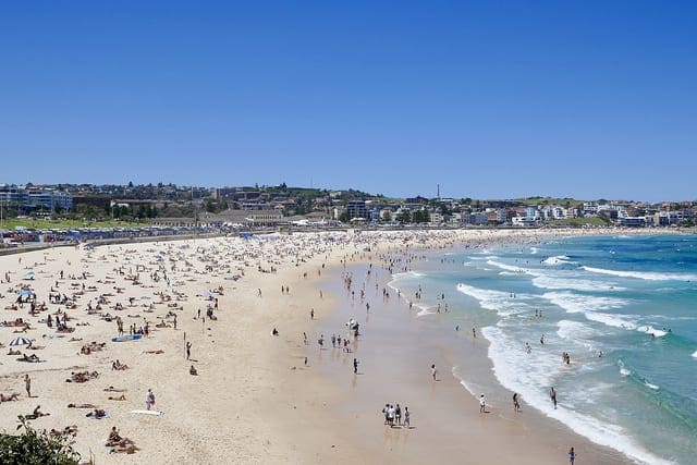
Next, download a photograph of Bondi Beach in Sydney Australia, taken by Isabell Schulz and released under a permissive license. Save the image in your current working directory with the filename ‘bondi_beach.jpg‘.
Next, we can use the Pillow library to load the photo, confirm the min and max pixel values, normalize the values, and confirm the normalization was performed.
# example of pixel normalization
from numpy import asarray
from PIL import Image
# load image
image = Image.open('bondi_beach.jpg')
pixels = asarray(image)
# confirm pixel range is 0-255
print('Data Type: %s' % pixels.dtype)
print('Min: %.3f, Max: %.3f' % (pixels.min(), pixels.max()))
# convert from integers to floats
pixels = pixels.astype('float32')
# normalize to the range 0-1
pixels /= 255.0
# confirm the normalization
print('Min: %.3f, Max: %.3f' % (pixels.min(), pixels.max()))
Your Task
Your task in this lesson is to run the example code on the provided photograph and report the min and max pixel values before and after the normalization.
For bonus points, you can update the example to standardize the pixel values.
Post your findings in the comments below. I would love to see what you discover.
In the next lesson, you will discover information about convolutional neural network models.
Lesson 03: Convolutional Neural Networks
In this lesson, you will discover how to construct a convolutional neural network using a convolutional layer, pooling layer, and fully connected output layer.
Convolutional Layers
A convolution is the simple application of a filter to an input that results in an activation. Repeated application of the same filter to an input results in a map of activations called a feature map, indicating the locations and strength of a detected feature in an input, such as an image.
A convolutional layer can be created by specifying both the number of filters to learn and the fixed size of each filter, often called the kernel shape.
Pooling Layers
Pooling layers provide an approach to downsampling feature maps by summarizing the presence of features in patches of the feature map.
Maximum pooling, or max pooling, is a pooling operation that calculates the maximum, or largest, value in each patch of each feature map.
Classifier Layer
Once the features have been extracted, they can be interpreted and used to make a prediction, such as classifying the type of object in a photograph.
This can be achieved by first flattening the two-dimensional feature maps, and then adding a fully connected output layer. For a binary classification problem, the output layer would have one node that would predict a value between 0 and 1 for the two classes.
Convolutional Neural Network
The example below creates a convolutional neural network that expects grayscale images with the square size of 256×256 pixels, with one convolutional layer with 32 filters, each with the size of 3×3 pixels, a max pooling layer, and a binary classification output layer.
# cnn with single convolutional, pooling and output layer
from keras.models import Sequential
from keras.layers import Conv2D
from keras.layers import MaxPooling2D
from keras.layers import Flatten
from keras.layers import Dense
# create model
model = Sequential()
# add convolutional layer
model.add(Conv2D(32, (3,3), input_shape=(256, 256, 1)))
model.add(MaxPooling2D())
model.add(Flatten())
model.add(Dense(1, activation='sigmoid'))
model.summary()
Your Task
Your task in this lesson is to run the example and describe how the shape of an input image would be changed by the convolutional and pooling layers.
For extra points, you could try adding more convolutional or pooling layers and describe the effect it has on the image as it flows through the model.
Post your findings in the comments below. I would love to see what you discover.
In the next lesson, you will learn how to use a deep convolutional neural network to classify photographs of objects.
Lesson 04: Image Classification
In this lesson, you will discover how to use a pre-trained model to classify photographs of objects.
Deep convolutional neural network models may take days, or even weeks, to train on very large datasets.
A way to short-cut this process is to re-use the model weights from pre-trained models that were developed for standard computer vision benchmark datasets, such as the ImageNet image recognition tasks.
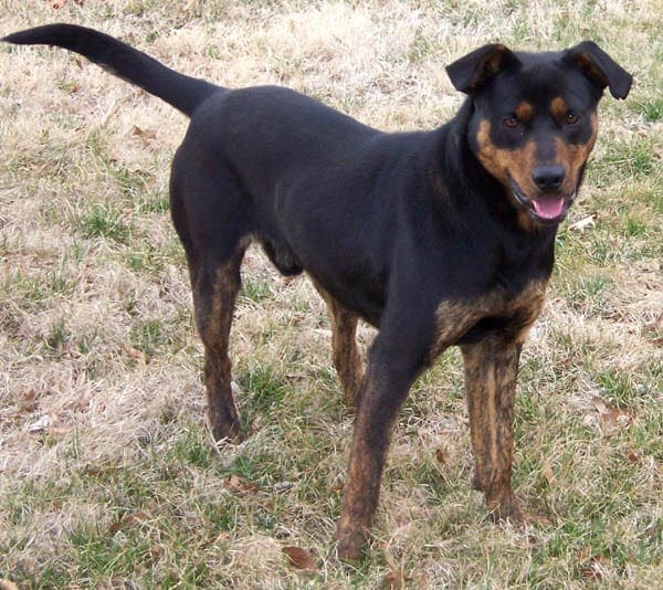
The example below uses the VGG-16 pre-trained model to classify photographs of objects into one of 1,000 known classes.
Download this photograph of a dog taken by Justin Morgan and released under a permissive license. Save it in your current working directory with the filename ‘dog.jpg‘.
The example below will load the photograph and output a prediction, classifying the object in the photograph.
Note: The first time you run the example, the pre-trained model will have to be downloaded, which is a few hundred megabytes and make take a few minutes based on the speed of your internet connection.
# example of using a pre-trained model as a classifier
from keras.preprocessing.image import load_img
from keras.preprocessing.image import img_to_array
from keras.applications.vgg16 import preprocess_input
from keras.applications.vgg16 import decode_predictions
from keras.applications.vgg16 import VGG16
# load an image from file
image = load_img('dog.jpg', target_size=(224, 224))
# convert the image pixels to a numpy array
image = img_to_array(image)
# reshape data for the model
image = image.reshape((1, image.shape[0], image.shape[1], image.shape[2]))
# prepare the image for the VGG model
image = preprocess_input(image)
# load the model
model = VGG16()
# predict the probability across all output classes
yhat = model.predict(image)
# convert the probabilities to class labels
label = decode_predictions(yhat)
# retrieve the most likely result, e.g. highest probability
label = label[0][0]
# print the classification
print('%s (%.2f%%)' % (label[1], label[2]*100))
Your Task
Your task in this lesson is to run the example and report the result.
For bonus points, try running the example on another photograph of a common object.
Post your findings in the comments below. I would love to see what you discover.
In the next lesson, you will discover how to fit and evaluate a model for image classification.
Lesson 05: Train Image Classification Model
In this lesson, you will discover how to train and evaluate a convolutional neural network for image classification.
The Fashion-MNIST clothing classification problem is a new standard dataset used in computer vision and deep learning.
It is a dataset comprised of 60,000 small square 28×28 pixel grayscale images of items of 10 types of clothing, such as shoes, t-shirts, dresses, and more.
The example below loads the dataset, scales the pixel values, then fits a convolutional neural network on the training dataset and evaluates the performance of the network on the test dataset.
The example will run in just a few minutes on a modern CPU; no GPU is required.
# fit a cnn on the fashion mnist dataset
from keras.datasets import fashion_mnist
from keras.utils import to_categorical
from keras.models import Sequential
from keras.layers import Conv2D
from keras.layers import MaxPooling2D
from keras.layers import Dense
from keras.layers import Flatten
# load dataset
(trainX, trainY), (testX, testY) = fashion_mnist.load_data()
# reshape dataset to have a single channel
trainX = trainX.reshape((trainX.shape[0], 28, 28, 1))
testX = testX.reshape((testX.shape[0], 28, 28, 1))
# convert from integers to floats
trainX, testX = trainX.astype('float32'), testX.astype('float32')
# normalize to range 0-1
trainX,testX  = trainX / 255.0, testX / 255.0
# one hot encode target values
trainY, testY = to_categorical(trainY), to_categorical(testY)
# define model
model = Sequential()
model.add(Conv2D(32, (3, 3), activation='relu', kernel_initializer='he_uniform', input_shape=(28, 28, 1)))
model.add(MaxPooling2D())
model.add(Flatten())
model.add(Dense(100, activation='relu', kernel_initializer='he_uniform'))
model.add(Dense(10, activation='softmax'))
model.compile(optimizer='adam', loss='categorical_crossentropy', metrics=['accuracy'])
# fit model
model.fit(trainX, trainY, epochs=10, batch_size=32, verbose=2)
# evaluate model
loss, acc = model.evaluate(testX, testY, verbose=0)
print(loss, acc)
Your Task
Your task in this lesson is to run the example and report the performance of the model on the test dataset.
For bonus points, try varying the configuration of the model, or try saving the model and later loading it and using it to make a prediction on new grayscale photographs of clothing.
Post your findings in the comments below. I would love to see what you discover.
In the next lesson, you will discover how to use image augmentation on training data.
Lesson 06: Image Augmentation
In this lesson, you will discover how to use image augmentation.
Image data augmentation is a technique that can be used to artificially expand the size of a training dataset by creating modified versions of images in the dataset.
Training deep learning neural network models on more data can result in more skillful models, and the augmentation techniques can create variations of the images that can improve the ability of the fit models to generalize what they have learned to new images.
The Keras deep learning neural network library provides the capability to fit models using image data augmentation via the ImageDataGenerator class.
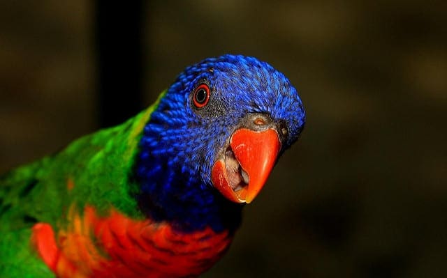
Download a photograph of a bird by AndYaDontStop, released under a permissive license. Save it into your current working directory with the name ‘bird.jpg‘.
The example below will load the photograph as a dataset and use image augmentation to create flipped and rotated versions of the image that can be used to train a convolutional neural network model.
# example using image augmentation
from numpy import expand_dims
from keras.preprocessing.image import load_img
from keras.preprocessing.image import img_to_array
from keras.preprocessing.image import ImageDataGenerator
from matplotlib import pyplot
# load the image
img = load_img('bird.jpg')
# convert to numpy array
data = img_to_array(img)
# expand dimension to one sample
samples = expand_dims(data, 0)
# create image data augmentation generator
datagen = ImageDataGenerator(horizontal_flip=True, vertical_flip=True, rotation_range=90)
# prepare iterator
it = datagen.flow(samples, batch_size=1)
# generate samples and plot
for i in range(9):
     # define subplot
     pyplot.subplot(330 + 1 + i)
     # generate batch of images
     batch = it.next()
     # convert to unsigned integers for viewing
     image = batch[0].astype('uint32')
     # plot raw pixel data
     pyplot.imshow(image)
# show the figure
pyplot.show()
Your Task
Your task in this lesson is to run the example and report the effect that the image augmentation has had on the original image.
For bonus points, try additional types of image augmentation, supported by the ImageDataGenerator class.
Post your findings in the comments below. I would love to see what you find.
In the next lesson, you will discover how to use a deep convolutional network to detect faces in photographs.
Lesson 07: Face Detection
In this lesson, you will discover how to use a convolutional neural network for face detection.
Face detection is a trivial problem for humans to solve and has been solved reasonably well by classical feature-based techniques, such as the cascade classifier.
More recently, deep learning methods have achieved state-of-the-art results on standard face detection datasets. One example is the Multi-task Cascade Convolutional Neural Network, or MTCNN for short.
The ipazc/MTCNN project provides an open source implementation of the MTCNN that can be installed easily as follows:
sudo pip install mtcnn
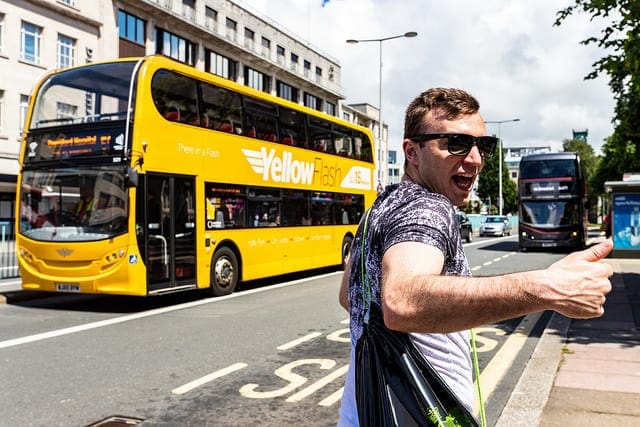
Download a photograph of a person on the street taken by Holland and released under a permissive license. Save it into your current working directory with the name ‘street.jpg‘.
The example below will load the photograph and use the MTCNN model to detect faces and will plot the photo and draw a box around the first detected face.
# face detection with mtcnn on a photograph
from matplotlib import pyplot
from matplotlib.patches import Rectangle
from mtcnn.mtcnn import MTCNN
# load image from file
pixels = pyplot.imread('street.jpg')
# create the detector, using default weights
detector = MTCNN()
# detect faces in the image
faces = detector.detect_faces(pixels)
# plot the image
pyplot.imshow(pixels)
# get the context for drawing boxes
ax = pyplot.gca()
# get coordinates from the first face
x, y, width, height = faces[0]['box']
# create the shape
rect = Rectangle((x, y), width, height, fill=False, color='red')
# draw the box
ax.add_patch(rect)
# show the plot
pyplot.show()
Your Task
Your task in this lesson is to run the example and describe the result.
For bonus points, try the model on another photograph with multiple faces and update the code example to draw a box around each detected face.
Post your findings in the comments below. I would love to see what you discover.
The End!
(Look How Far You Have Come)
You made it. Well done!
Take a moment and look back at how far you have come.
You discovered:
- What computer vision is and the promise and impact that deep learning is having on the field.
- How to scale the pixel values of image data in order to make them ready for modeling.
- How to develop a convolutional neural network model from scratch.
- How to use a pre-trained model to classify photographs of objects.
- How to train a model from scratch to classify photographs of clothing.
- How to use image augmentation to create modified copies of photographs in your training dataset.
- How to use a pre-trained deep learning model to detect people’s faces in photographs.
This is just the beginning of your journey with deep learning for computer vision. Keep practicing and developing your skills.
Take the next step and check out my book on deep learning for computer vision.
Summary
How Did You Do With The Mini-Course?
Did you enjoy this crash course?
Do you have any questions? Were there any sticking points?
Let me know. Leave a comment below.
The post How to Get Started With Deep Learning for Computer Vision (7-Day Mini-Course) appeared first on Machine Learning Mastery.