Author: Jason Brownlee
Deep convolutional neural network models may take days or even weeks to train on very large datasets.
A way to short-cut this process is to re-use the model weights from pre-trained models that were developed for standard computer vision benchmark datasets, such as the ImageNet image recognition tasks. Top performing models can be downloaded and used directly, or integrated into a new model for your own computer vision problems.
In this post, you will discover how to use transfer learning when developing convolutional neural networks for computer vision applications.
After reading this post, you will know:
- Transfer learning involves using models trained on one problem as a starting point on a related problem.
- Transfer learning is flexible, allowing the use of pre-trained models directly, as feature extraction preprocessing, and integrated into entirely new models.
- Keras provides convenient access to many top performing models on the ImageNet image recognition tasks such as VGG, Inception, and ResNet.
Let’s get started.
How to Use Transfer Learning when Developing Convolutional Neural Network Models
Photo by GoToVan, some rights reserved.
Overview
This tutorial is divided into five parts; they are:
- What Is Transfer Learning?
- Transfer Learning for Image Recognition
- How to Use Pre-Trained Models
- Models for Transfer Learning
- Examples of Using Pre-Trained Models
What Is Transfer Learning?
Transfer learning generally refers to a process where a model trained on one problem is used in some way on a second related problem.
In deep learning, transfer learning is a technique whereby a neural network model is first trained on a problem similar to the problem that is being solved. One or more layers from the trained model are then used in a new model trained on the problem of interest.
This is typically understood in a supervised learning context, where the input is the same but the target may be of a different nature. For example, we may learn about one set of visual categories, such as cats and dogs, in the first setting, then learn about a different set of visual categories, such as ants and wasps, in the second setting.
— Page 536, Deep Learning, 2016.
Transfer learning has the benefit of decreasing the training time for a neural network model and can result in lower generalization error.
The weights in re-used layers may be used as the starting point for the training process and adapted in response to the new problem. This usage treats transfer learning as a type of weight initialization scheme. This may be useful when the first related problem has a lot more labeled data than the problem of interest and the similarity in the structure of the problem may be useful in both contexts.
… the objective is to take advantage of data from the first setting to extract information that may be useful when learning or even when directly making predictions in the second setting.
— Page 538, Deep Learning, 2016.
Want Results with Deep Learning for Computer Vision?
Take my free 7-day email crash course now (with sample code).
Click to sign-up and also get a free PDF Ebook version of the course.
Transfer Learning for Image Recognition
A range of high-performing models have been developed for image classification and demonstrated on the annual ImageNet Large Scale Visual Recognition Challenge, or ILSVRC.
This challenge, often referred to simply as ImageNet, given the source of the image used in the competition, has resulted in a number of innovations in the architecture and training of convolutional neural networks. In addition, many of the models used in the competitions have been released under a permissive license.
These models can be used as the basis for transfer learning in computer vision applications.
This is desirable for a number of reasons, not least:
- Useful Learned Features: The models have learned how to detect generic features from photographs, given that they were trained on more than 1,000,000 images for 1,000 categories.
- State-of-the-Art Performance: The models achieved state of the art performance and remain effective on the specific image recognition task for which they were developed.
- Easily Accessible: The model weights are provided as free downloadable files and many libraries provide convenient APIs to download and use the models directly.
The model weights can be downloaded and used in the same model architecture using a range of different deep learning libraries, including Keras.
How to Use Pre-Trained Models
The use of a pre-trained model is limited only by your creativity.
For example, a model may be downloaded and used as-is, such as embedded into an application and used to classify new photographs.
Alternately, models may be downloaded and use as feature extraction models. Here, the output of the model from a layer prior to the output layer of the model is used as input to a new classifier model.
Recall that convolutional layers closer to the input layer of the model learn low-level features such as lines, that layers in the middle of the layer learn complex abstract features that combine the lower level features extracted from the input, and layers closer to the output interpret the extracted features in the context of a classification task.
Armed with this understanding, a level of detail for feature extraction from an existing pre-trained model can be chosen. For example, if a new task is quite different from classifying objects in photographs (e.g. different to ImageNet), then perhaps the output of the pre-trained model after the few layers would be appropriate. If a new task is quite similar to the task of classifying objects in photographs, then perhaps the output from layers much deeper in the model can be used, or even the output of the fully connected layer prior to the output layer can be used.
The pre-trained model can be used as a separate feature extraction program, in which case input can be pre-processed by the model or portion of the model to a given an output (e.g. vector of numbers) for each input image, that can then use as input when training a new model.
Alternately, the pre-trained model or desired portion of the model can be integrated directly into a new neural network model. In this usage, the weights of the pre-trained can be frozen so that they are not updated as the new model is trained. Alternately, the weights may be updated during the training of the new model, perhaps with a lower learning rate, allowing the pre-trained model to act like a weight initialization scheme when training the new model.
We can summarize some of these usage patterns as follows:
- Classifier: The pre-trained model is used directly to classify new images.
- Standalone Feature Extractor: The pre-trained model, or some portion of the model, is used to pre-process images and extract relevant features.
- Integrated Feature Extractor: The pre-trained model, or some portion of the model, is integrated into a new model, but layers of the pre-trained model are frozen during training.
- Weight Initialization: The pre-trained model, or some portion of the model, is integrated into a new model, and the layers of the pre-trained model are trained in concert with the new model.
Each approach can be effective and save significant time in developing and training a deep convolutional neural network model.
It may not be clear as to which usage of the pre-trained model may yield the best results on your new computer vision task, therefore some experimentation may be required.
Models for Transfer Learning
There are perhaps a dozen or more top-performing models for image recognition that can be downloaded and used as the basis for image recognition and related computer vision tasks.
Perhaps three of the more popular models are as follows:
- VGG (e.g. VGG16 or VGG19).
- GoogLeNet (e.g. InceptionV3).
- Residual Network (e.g. ResNet50).
These models are both widely used for transfer learning both because of their performance, but also because they were examples that introduced specific architectural innovations, namely consistent and repeating structures (VGG), inception modules (GoogLeNet), and residual modules (ResNet).
Keras provides access to a number of top-performing pre-trained models that were developed for image recognition tasks.
They are available via the Applications API, and include functions to load a model with or without the pre-trained weights, and prepare data in a way that a given model may expect (e.g. scaling of size and pixel values).
The first time a pre-trained model is loaded, Keras will download the required model weights, which may take some time given the speed of your internet connection. Weights are stored in the .keras/models/ directory under your home directory and will be loaded from this location the next time that they are used.
When loading a given model, the “include_top” argument can be set to False, in which case the fully-connected output layers of the model used to make predictions is not loaded, allowing a new output layer to be added and trained. For example:
...
# load model without output layer
model = VGG16(include_top=False)
Additionally, when the “include_top” argument is False, the “input_tensor” argument must be specified, allowing the expected fixed-sized input of the model to be changed. For example:
...
# load model and specify a new input shape for images
new_input = Input(shape=(640, 480, 3))
model = VGG16(include_top=False, input_tensor=new_input)
A model without a top will output activations from the last convolutional or pooling layer directly. One approach to summarizing these activations for thier use in a classifier or as a feature vector representation of input is to add a global pooling layer, such as a max global pooling or average global pooling. The result is a vector that can be used as a feature descriptor for an input. Keras provides this capability directly via the ‘pooling‘ argument that can be set to ‘avg‘ or ‘max‘. For example:
...
# load model and specify a new input shape for images and avg pooling output
new_input = Input(shape=(640, 480, 3))
model = VGG16(include_top=False, input_tensor=new_input, pooling='avg')
Images can be prepared for a given model using the preprocess_input() function; e.g., pixel scaling is performed in a way that was performed to images in the training dataset when the model was developed. For example:
...
# prepare an image
from keras.applications.vgg16 import preprocess_input
images = ...
prepared_images = preprocess_input(images)
Finally, you may wish to use a model architecture on your dataset, but not use the pre-trained weights, and instead initialize the model with random weights and train the model from scratch.
This can be achieved by setting the ‘weights‘ argument to None instead of the default ‘imagenet‘. Additionally, the ‘classes‘ argument can be set to define the number of classes in your dataset, which will then be configured for you in the output layer of the model. For example:
...
# define a new model with random weights and 10 classes
new_input = Input(shape=(640, 480, 3))
model = VGG16(weights=None, input_tensor=new_input, classes=10)
Now that we are familiar with the API, let’s take a look at loading three models using the Keras Applications API.
Load the VGG16 Pre-trained Model
The VGG16 model was developed by the Visual Graphics Group (VGG) at Oxford and was described in the 2014 paper titled “Very Deep Convolutional Networks for Large-Scale Image Recognition.”
By default, the model expects color input images to be rescaled to the size of 224×224 squares.
The model can be loaded as follows:
# example of loading the vgg16 model
from keras.applications.vgg16 import VGG16
# load model
model = VGG16()
# summarize the model
model.summary()
Running the example will load the VGG16 model and download the model weights if required.
The model can then be used directly to classify a photograph into one of 1,000 classes. In this case, the model architecture is summarized to confirm that it was loaded correctly.
_________________________________________________________________
Layer (type)                 Output Shape              Param #
=================================================================
input_1 (InputLayer)         (None, 224, 224, 3)       0
_________________________________________________________________
block1_conv1 (Conv2D)        (None, 224, 224, 64)      1792
_________________________________________________________________
block1_conv2 (Conv2D)        (None, 224, 224, 64)      36928
_________________________________________________________________
block1_pool (MaxPooling2D)   (None, 112, 112, 64)      0
_________________________________________________________________
block2_conv1 (Conv2D)        (None, 112, 112, 128)     73856
_________________________________________________________________
block2_conv2 (Conv2D)        (None, 112, 112, 128)     147584
_________________________________________________________________
block2_pool (MaxPooling2D)   (None, 56, 56, 128)       0
_________________________________________________________________
block3_conv1 (Conv2D)        (None, 56, 56, 256)       295168
_________________________________________________________________
block3_conv2 (Conv2D)        (None, 56, 56, 256)       590080
_________________________________________________________________
block3_conv3 (Conv2D)        (None, 56, 56, 256)       590080
_________________________________________________________________
block3_pool (MaxPooling2D)   (None, 28, 28, 256)       0
_________________________________________________________________
block4_conv1 (Conv2D)        (None, 28, 28, 512)       1180160
_________________________________________________________________
block4_conv2 (Conv2D)        (None, 28, 28, 512)       2359808
_________________________________________________________________
block4_conv3 (Conv2D)        (None, 28, 28, 512)       2359808
_________________________________________________________________
block4_pool (MaxPooling2D)   (None, 14, 14, 512)       0
_________________________________________________________________
block5_conv1 (Conv2D)        (None, 14, 14, 512)       2359808
_________________________________________________________________
block5_conv2 (Conv2D)        (None, 14, 14, 512)       2359808
_________________________________________________________________
block5_conv3 (Conv2D)        (None, 14, 14, 512)       2359808
_________________________________________________________________
block5_pool (MaxPooling2D)   (None, 7, 7, 512)         0
_________________________________________________________________
flatten (Flatten)            (None, 25088)             0
_________________________________________________________________
fc1 (Dense)                  (None, 4096)              102764544
_________________________________________________________________
fc2 (Dense)                  (None, 4096)              16781312
_________________________________________________________________
predictions (Dense)          (None, 1000)              4097000
=================================================================
Total params: 138,357,544
Trainable params: 138,357,544
Non-trainable params: 0
_________________________________________________________________
Load the InceptionV3 Pre-Trained Model
The InceptionV3 is the third iteration of the inception architecture, first developed for the GoogLeNet model.
This model was developed by researchers at Google and described in the 2015 paper titled “Rethinking the Inception Architecture for Computer Vision.”
The model expects color images to have the square shape 299×299.
The model can be loaded as follows:
# example of loading the inception v3 model
from keras.applications.inception_v3 import InceptionV3
# load model
model = InceptionV3()
# summarize the model
model.summary()
Running the example will load the model, downloading the weights if required, and then summarize the model architecture to confirm it was loaded correctly.
The output is omitted in this case for brevity, as it is a deep model with many layers.
Load the ResNet50 Pre-trained Model
The Residual Network, or ResNet for short, is a model that makes use of the residual module involving shortcut connections.
It was developed by researchers at Microsoft and described in the 2015 paper titled “Deep Residual Learning for Image Recognition.”
The model expects color images to have the square shape 224×224.
# example of loading the resnet50 model
from keras.applications.resnet50 import ResNet50
# load model
model = ResNet50()
# summarize the model
model.summary()
Running the example will load the model, downloading the weights if required, and then summarize the model architecture to confirm it was loaded correctly.
The output is omitted in this case for brevity, as it is a deep model.
Examples of Using Pre-Trained Models
Now that we are familiar with how to load pre-trained models in Keras, let’s look at some examples of how they might be used in practice.
In these examples, we will work with the VGG16 model as it is a relatively straightforward model to use and a simple model architecture to understand.
We also need a photograph to work with in these examples. Below is a photograph of a dog, taken by Justin Morgan and made available under a permissive license.
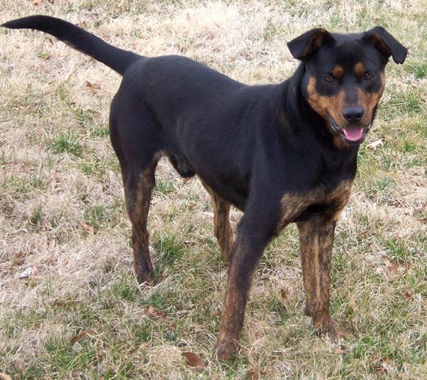
Photograph of a Dog
Download the photograph and place it in your current working directory with the filename ‘dog.jpg‘.
Pre-Trained Model as Classifier
A pre-trained model can be used directly to classify new photographs as one of the 1,000 known classes in the image classification task in the ILSVRC.
We will use the VGG16 model to classify new images.
First, the photograph needs to loaded and reshaped to a 224×224 square, expected by the model, and the pixel values scaled in the way expected by the model. The model operates on an array of samples, therefore the dimensions of a loaded image need to be expanded by 1, for one image with 224×224 pixels and three channels.
# load an image from file
image = load_img('dog.jpg', target_size=(224, 224))
# convert the image pixels to a numpy array
image = img_to_array(image)
# reshape data for the model
image = image.reshape((1, image.shape[0], image.shape[1], image.shape[2]))
# prepare the image for the VGG model
image = preprocess_input(image)
Next, the model can be loaded and a prediction made.
This means that a predicted probability of the photo belonging to each of the 1,000 classes is made. In this example, we are only concerned with the most likely class, so we can decode the predictions and retrieve the label or name of the class with the highest probability.
# predict the probability across all output classes
yhat = model.predict(image)
# convert the probabilities to class labels
label = decode_predictions(yhat)
# retrieve the most likely result, e.g. highest probability
label = label[0][0]
Tying all of this together, the complete example below loads a new photograph and predicts the most likely class.
# example of using a pre-trained model as a classifier
from keras.preprocessing.image import load_img
from keras.preprocessing.image import img_to_array
from keras.applications.vgg16 import preprocess_input
from keras.applications.vgg16 import decode_predictions
from keras.applications.vgg16 import VGG16
# load an image from file
image = load_img('dog.jpg', target_size=(224, 224))
# convert the image pixels to a numpy array
image = img_to_array(image)
# reshape data for the model
image = image.reshape((1, image.shape[0], image.shape[1], image.shape[2]))
# prepare the image for the VGG model
image = preprocess_input(image)
# load the model
model = VGG16()
# predict the probability across all output classes
yhat = model.predict(image)
# convert the probabilities to class labels
label = decode_predictions(yhat)
# retrieve the most likely result, e.g. highest probability
label = label[0][0]
# print the classification
print('%s (%.2f%%)' % (label[1], label[2]*100))
Running the example predicts more than just dog; it also predicts the specific breed of ‘Doberman‘ with a probability of 33.59%, which may, in fact, be correct.
Doberman (33.59%)
Pre-Trained Model as Feature Extractor Preprocessor
The pre-trained model may be used as a standalone program to extract features from new photographs.
Specifically, the extracted features of a photograph may be a vector of numbers that the model will use to describe the specific features in a photograph. These features can then be used as input in the development of a new model.
The last few layers of the VGG16 model are fully connected layers prior to the output layer. These layers will provide a complex set of features to describe a given input image and may provide useful input when training a new model for image classification or related computer vision task.
The image can be loaded and prepared for the model, as we did before in the previous example.
We will load the model with the classifier output part of the model, but manually remove the final output layer. This means that the second last fully connected layer with 4,096 nodes will be the new output layer.
# load model
model = VGG16()
# remove the output layer
model.layers.pop()
model = Model(inputs=model.inputs, outputs=model.layers[-1].output)
This vector of 4,096 numbers will be used to represent the complex features of a given input image that can then be saved to file to be loaded later and used as input to train a new model. We can save it as a pickle file.
# get extracted features
features = model.predict(image)
print(features.shape)
# save to file
dump(features, open('dog.pkl', 'wb'))
Tying all of this together, the complete example of using the model as a standalone feature extraction model is listed below.
# example of using the vgg16 model as a feature extraction model
from keras.preprocessing.image import load_img
from keras.preprocessing.image import img_to_array
from keras.applications.vgg16 import preprocess_input
from keras.applications.vgg16 import decode_predictions
from keras.applications.vgg16 import VGG16
from keras.models import Model
from pickle import dump
# load an image from file
image = load_img('dog.jpg', target_size=(224, 224))
# convert the image pixels to a numpy array
image = img_to_array(image)
# reshape data for the model
image = image.reshape((1, image.shape[0], image.shape[1], image.shape[2]))
# prepare the image for the VGG model
image = preprocess_input(image)
# load model
model = VGG16()
# remove the output layer
model.layers.pop()
model = Model(inputs=model.inputs, outputs=model.layers[-1].output)
# get extracted features
features = model.predict(image)
print(features.shape)
# save to file
dump(features, open('dog.pkl', 'wb'))
Running the example loads the photograph, then prepares the model as a feature extraction model.
The features are extracted from the loaded photo and the shape of the feature vector is printed, showing it has 4,096 numbers. This feature is then saved to a new file dog.pkl in the current working directory.
(1, 4096)
This process could be repeated for each photo in a new training dataset.
Pre-Trained Model as Feature Extractor in Model
We can use some or all of the layers in a pre-trained model as a feature extraction component of a new model directly.
This can be achieved by loading the model, then simply adding new layers. This may involve adding new convolutional and pooling layers to expand upon the feature extraction capabilities of the model or adding new fully connected classifier type layers to learn how to interpret the extracted features on a new dataset, or some combination.
For example, we can load the VGG16 models without the classifier part of the model by specifying the “include_top” argument to “False”, and specify the preferred shape of the images in our new dataset as 300×300.
# load model without classifier layers
model = VGG16(include_top=False, input_shape=(224, 224, 3))
We can then use the Keras function API to add a new Flatten layer after the last pooling layer in the VGG16 model, then define a new classifier model with a Dense fully connected layer and an output layer that will predict the probability for 10 classes.
# add new classifier layers
flat1 = Flatten()(model.outputs)
class1 = Dense(1024, activation='relu')(flat1)
output = Dense(10, activation='softmax')(class1)
# define new model
model = Model(inputs=model.inputs, outputs=output)
An alternative approach to adding a Flatten layer would be to define the VGG16 model with an average pooling layer, and then add fully connected layers. Perhaps try both approaches on your application and see which results in the best performance.
The weights of the VGG16 model and the weights for the new model will all be trained together on the new dataset.
The complete example is listed below.
# example of tending the vgg16 model
from keras.applications.vgg16 import VGG16
from keras.models import Model
from keras.layers import Dense
from keras.layers import Flatten
# load model without classifier layers
model = VGG16(include_top=False, input_shape=(300, 300, 3))
# add new classifier layers
flat1 = Flatten()(model.outputs)
class1 = Dense(1024, activation='relu')(flat1)
output = Dense(10, activation='softmax')(class1)
# define new model
model = Model(inputs=model.inputs, outputs=output)
# summarize
model.summary()
# ...
Running the example defines the new model ready for training and summarizes the model architecture.
We can see that we have flattened the output of the last pooling layer and added our new fully connected layers.
_________________________________________________________________
Layer (type)                 Output Shape              Param #
=================================================================
input_1 (InputLayer)         (None, 300, 300, 3)       0
_________________________________________________________________
block1_conv1 (Conv2D)        (None, 300, 300, 64)      1792
_________________________________________________________________
block1_conv2 (Conv2D)        (None, 300, 300, 64)      36928
_________________________________________________________________
block1_pool (MaxPooling2D)   (None, 150, 150, 64)      0
_________________________________________________________________
block2_conv1 (Conv2D)        (None, 150, 150, 128)     73856
_________________________________________________________________
block2_conv2 (Conv2D)        (None, 150, 150, 128)     147584
_________________________________________________________________
block2_pool (MaxPooling2D)   (None, 75, 75, 128)       0
_________________________________________________________________
block3_conv1 (Conv2D)        (None, 75, 75, 256)       295168
_________________________________________________________________
block3_conv2 (Conv2D)        (None, 75, 75, 256)       590080
_________________________________________________________________
block3_conv3 (Conv2D)        (None, 75, 75, 256)       590080
_________________________________________________________________
block3_pool (MaxPooling2D)   (None, 37, 37, 256)       0
_________________________________________________________________
block4_conv1 (Conv2D)        (None, 37, 37, 512)       1180160
_________________________________________________________________
block4_conv2 (Conv2D)        (None, 37, 37, 512)       2359808
_________________________________________________________________
block4_conv3 (Conv2D)        (None, 37, 37, 512)       2359808
_________________________________________________________________
block4_pool (MaxPooling2D)   (None, 18, 18, 512)       0
_________________________________________________________________
block5_conv1 (Conv2D)        (None, 18, 18, 512)       2359808
_________________________________________________________________
block5_conv2 (Conv2D)        (None, 18, 18, 512)       2359808
_________________________________________________________________
block5_conv3 (Conv2D)        (None, 18, 18, 512)       2359808
_________________________________________________________________
block5_pool (MaxPooling2D)   (None, 9, 9, 512)         0
_________________________________________________________________
flatten_1 (Flatten)          (None, 41472)             0
_________________________________________________________________
dense_1 (Dense)              (None, 1024)              42468352
_________________________________________________________________
dense_2 (Dense)              (None, 10)                10250
=================================================================
Total params: 57,193,290
Trainable params: 57,193,290
Non-trainable params: 0
_________________________________________________________________
Alternately, we may wish to use the VGG16 model layers, but train the new layers of the model without updating the weights of the VGG16 layers. This will allow the new output layers to learn to interpret the learned features of the VGG16 model.
This can be achieved by setting the “trainable” property on each of the layers in the loaded VGG model to False prior to training. For example:
# load model without classifier layers
model = VGG16(include_top=False, input_shape=(300, 300, 3))
# mark loaded layers as not trainable
for layer in model.layers:
	layer.trainable = False
...
You can pick and choose which layers are trainable.
For example, perhaps you want to retrain some of the convolutional layers deep in the model, but none of the layers earlier in the model. For example:
# load model without classifier layers
model = VGG16(include_top=False, input_shape=(300, 300, 3))
# mark some layers as not trainable
model.get_layer('block1_conv1').trainable = False
model.get_layer('block1_conv2').trainable = False
model.get_layer('block2_conv1').trainable = False
model.get_layer('block2_conv2').trainable = False
...
Further Reading
This section provides more resources on the topic if you are looking to go deeper.
Posts
- How to Improve Performance With Transfer Learning for Deep Learning Neural Networks
- A Gentle Introduction to Transfer Learning for Deep Learning
- How to Use The Pre-Trained VGG Model to Classify Objects in Photographs
Books
- Deep Learning, 2016.
Papers
- A Survey on Transfer Learning, 2010.
- How transferable are features in deep neural networks?, 2014.
- CNN features off-the-shelf: An astounding baseline for recognition, 2014.
APIs
Articles
Summary
In this post, you discovered how to use transfer learning when developing convolutional neural networks for computer vision applications.
Specifically, you learned:
- Transfer learning involves using models trained on one problem as a starting point on a related problem.
- Transfer learning is flexible, allowing the use of pre-trained models directly as feature extraction preprocessing and integrated into entirely new models.
- Keras provides convenient access to many top performing models on the ImageNet image recognition tasks such as VGG, Inception, and ResNet.
Do you have any questions?
Ask your questions in the comments below and I will do my best to answer.
The post How to Use Transfer Learning when Developing Convolutional Neural Network Models appeared first on Machine Learning Mastery.