
Author: Jason Brownlee
Object detection is a task in computer vision that involves identifying the presence, location, and type of one or more objects in a given photograph.
It is a challenging problem that involves building upon methods for object recognition (e.g. where are they), object localization (e.g. what are their extent), and object classification (e.g. what are they).
In recent years, deep learning techniques are achieving state-of-the-art results for object detection, such as on standard benchmark datasets and in computer vision competitions. Notable is the “You Only Look Once,” or YOLO, family of Convolutional Neural Networks that achieve near state-of-the-art results with a single end-to-end model that can perform object detection in real-time.
In this tutorial, you will discover how to develop a YOLOv3 model for object detection on new photographs.
After completing this tutorial, you will know:
- YOLO-based Convolutional Neural Network family of models for object detection and the most recent variation called YOLOv3.
- The best-of-breed open source library implementation of the YOLOv3 for the Keras deep learning library.
- How to use a pre-trained YOLOv3 to perform object localization and detection on new photographs.
Let’s get started.
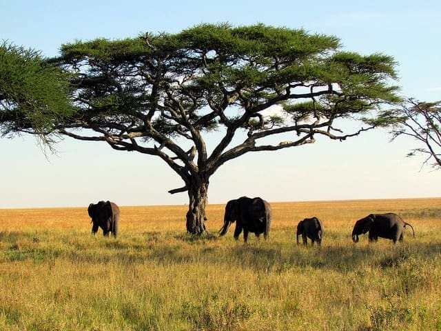
How to Perform Object Detection With YOLOv3 in Keras
Photo by David Berkowitz, some rights reserved.
Tutorial Overview
This tutorial is divided into three parts; they are:
- YOLO for Object Detection
- Experiencor YOLO3 Project
- Object Detection With YOLOv3
Want Results with Deep Learning for Computer Vision?
Take my free 7-day email crash course now (with sample code).
Click to sign-up and also get a free PDF Ebook version of the course.
YOLO for Object Detection
Object detection is a computer vision task that involves both localizing one or more objects within an image and classifying each object in the image.
It is a challenging computer vision task that requires both successful object localization in order to locate and draw a bounding box around each object in an image, and object classification to predict the correct class of object that was localized.
The “You Only Look Once,” or YOLO, family of models are a series of end-to-end deep learning models designed for fast object detection, developed by Joseph Redmon, et al. and first described in the 2015 paper titled “You Only Look Once: Unified, Real-Time Object Detection.”
The approach involves a single deep convolutional neural network (originally a version of GoogLeNet, later updated and called DarkNet based on VGG) that splits the input into a grid of cells and each cell directly predicts a bounding box and object classification. The result is a large number of candidate bounding boxes that are consolidated into a final prediction by a post-processing step.
There are three main variations of the approach, at the time of writing; they are YOLOv1, YOLOv2, and YOLOv3. The first version proposed the general architecture, whereas the second version refined the design and made use of predefined anchor boxes to improve bounding box proposal, and version three further refined the model architecture and training process.
Although the accuracy of the models is close but not as good as Region-Based Convolutional Neural Networks (R-CNNs), they are popular for object detection because of their detection speed, often demonstrated in real-time on video or with camera feed input.
A single neural network predicts bounding boxes and class probabilities directly from full images in one evaluation. Since the whole detection pipeline is a single network, it can be optimized end-to-end directly on detection performance.
— You Only Look Once: Unified, Real-Time Object Detection, 2015.
In this tutorial, we will focus on using YOLOv3.
Experiencor YOLO3 for Keras Project
Source code for each version of YOLO is available, as well as pre-trained models.
The official DarkNet GitHub repository contains the source code for the YOLO versions mentioned in the papers, written in C. The repository provides a step-by-step tutorial on how to use the code for object detection.
It is a challenging model to implement from scratch, especially for beginners as it requires the development of many customized model elements for training and for prediction. For example, even using a pre-trained model directly requires sophisticated code to distill and interpret the predicted bounding boxes output by the model.
Instead of developing this code from scratch, we can use a third-party implementation. There are many third-party implementations designed for using YOLO with Keras, and none appear to be standardized and designed to be used as a library.
The YAD2K project was a de facto standard for YOLOv2 and provided scripts to convert the pre-trained weights into Keras format, use the pre-trained model to make predictions, and provided the code required to distill interpret the predicted bounding boxes. Many other third-party developers have used this code as a starting point and updated it to support YOLOv3.
Perhaps the most widely used project for using pre-trained the YOLO models is called “keras-yolo3: Training and Detecting Objects with YOLO3” by Huynh Ngoc Anh or experiencor. The code in the project has been made available under a permissive MIT open source license. Like YAD2K, it provides scripts to both load and use pre-trained YOLO models as well as transfer learning for developing YOLOv3 models on new datasets.
He also has a keras-yolo2 project that provides similar code for YOLOv2 as well as detailed tutorials on how to use the code in the repository. The keras-yolo3 project appears to be an updated version of that project.
Interestingly, experiencor has used the model as the basis for some experiments and trained versions of the YOLOv3 on standard object detection problems such as a kangaroo dataset, racoon dataset, red blood cell detection, and others. He has listed model performance, provided the model weights for download and provided YouTube videos of model behavior. For example:
We will use experiencor’s keras-yolo3 project as the basis for performing object detection with a YOLOv3 model in this tutorial.
In case the repository changes or is removed (which can happen with third-party open source projects), a fork of the code at the time of writing is provided.
Object Detection With YOLOv3
The keras-yolo3 project provides a lot of capability for using YOLOv3 models, including object detection, transfer learning, and training new models from scratch.
In this section, we will use a pre-trained model to perform object detection on an unseen photograph. This capability is available in a single Python file in the repository called “yolo3_one_file_to_detect_them_all.py” that has about 435 lines. This script is, in fact, a program that will use pre-trained weights to prepare a model and use that model to perform object detection and output a model. It also depends upon OpenCV.
Instead of using this program directly, we will reuse elements from this program and develop our own scripts to first prepare and save a Keras YOLOv3 model, and then load the model to make a prediction for a new photograph.
Create and Save Model
The first step is to download the pre-trained model weights.
These were trained using the DarkNet code base on the MSCOCO dataset. Download the model weights and place them into your current working directory with the filename “yolov3.weights.” It is a large file and may take a moment to download depending on the speed of your internet connection.
Next, we need to define a Keras model that has the right number and type of layers to match the downloaded model weights. The model architecture is called a “DarkNet” and was originally loosely based on the VGG-16 model.
The “yolo3_one_file_to_detect_them_all.py” script provides the make_yolov3_model() function to create the model for us, and the helper function _conv_block() that is used to create blocks of layers. These two functions can be copied directly from the script.
We can now define the Keras model for YOLOv3.
# define the model
model = make_yolov3_model()
Next, we need to load the model weights. The model weights are stored in whatever format that was used by DarkNet. Rather than trying to decode the file manually, we can use the WeightReader class provided in the script.
To use the WeightReader, it is instantiated with the path to our weights file (e.g. ‘yolov3.weights‘). This will parse the file and load the model weights into memory in a format that we can set into our Keras model.
# load the model weights
weight_reader = WeightReader('yolov3.weights')
We can then call the load_weights() function of the WeightReader instance, passing in our defined Keras model to set the weights into the layers.
# set the model weights into the model
weight_reader.load_weights(model)
That’s it; we now have a YOLOv3 model for use.
We can save this model to a Keras compatible .h5 model file ready for later use.
# save the model to file
model.save('model.h5')
We can tie all of this together; the complete code example including functions copied directly from the “yolo3_one_file_to_detect_them_all.py” script is listed below.
# create a YOLOv3 Keras model and save it to file
# based on https://github.com/experiencor/keras-yolo3
import struct
import numpy as np
from keras.layers import Conv2D
from keras.layers import Input
from keras.layers import BatchNormalization
from keras.layers import LeakyReLU
from keras.layers import ZeroPadding2D
from keras.layers import UpSampling2D
from keras.layers.merge import add, concatenate
from keras.models import Model

def _conv_block(inp, convs, skip=True):
	x = inp
	count = 0
	for conv in convs:
		if count == (len(convs) - 2) and skip:
			skip_connection = x
		count += 1
		if conv['stride'] > 1: x = ZeroPadding2D(((1,0),(1,0)))(x) # peculiar padding as darknet prefer left and top
		x = Conv2D(conv['filter'],
				   conv['kernel'],
				   strides=conv['stride'],
				   padding='valid' if conv['stride'] > 1 else 'same', # peculiar padding as darknet prefer left and top
				   name='conv_' + str(conv['layer_idx']),
				   use_bias=False if conv['bnorm'] else True)(x)
		if conv['bnorm']: x = BatchNormalization(epsilon=0.001, name='bnorm_' + str(conv['layer_idx']))(x)
		if conv['leaky']: x = LeakyReLU(alpha=0.1, name='leaky_' + str(conv['layer_idx']))(x)
	return add([skip_connection, x]) if skip else x

def make_yolov3_model():
	input_image = Input(shape=(None, None, 3))
	# Layer  0 => 4
	x = _conv_block(input_image, [{'filter': 32, 'kernel': 3, 'stride': 1, 'bnorm': True, 'leaky': True, 'layer_idx': 0},
								  {'filter': 64, 'kernel': 3, 'stride': 2, 'bnorm': True, 'leaky': True, 'layer_idx': 1},
								  {'filter': 32, 'kernel': 1, 'stride': 1, 'bnorm': True, 'leaky': True, 'layer_idx': 2},
								  {'filter': 64, 'kernel': 3, 'stride': 1, 'bnorm': True, 'leaky': True, 'layer_idx': 3}])
	# Layer  5 => 8
	x = _conv_block(x, [{'filter': 128, 'kernel': 3, 'stride': 2, 'bnorm': True, 'leaky': True, 'layer_idx': 5},
						{'filter':  64, 'kernel': 1, 'stride': 1, 'bnorm': True, 'leaky': True, 'layer_idx': 6},
						{'filter': 128, 'kernel': 3, 'stride': 1, 'bnorm': True, 'leaky': True, 'layer_idx': 7}])
	# Layer  9 => 11
	x = _conv_block(x, [{'filter':  64, 'kernel': 1, 'stride': 1, 'bnorm': True, 'leaky': True, 'layer_idx': 9},
						{'filter': 128, 'kernel': 3, 'stride': 1, 'bnorm': True, 'leaky': True, 'layer_idx': 10}])
	# Layer 12 => 15
	x = _conv_block(x, [{'filter': 256, 'kernel': 3, 'stride': 2, 'bnorm': True, 'leaky': True, 'layer_idx': 12},
						{'filter': 128, 'kernel': 1, 'stride': 1, 'bnorm': True, 'leaky': True, 'layer_idx': 13},
						{'filter': 256, 'kernel': 3, 'stride': 1, 'bnorm': True, 'leaky': True, 'layer_idx': 14}])
	# Layer 16 => 36
	for i in range(7):
		x = _conv_block(x, [{'filter': 128, 'kernel': 1, 'stride': 1, 'bnorm': True, 'leaky': True, 'layer_idx': 16+i*3},
							{'filter': 256, 'kernel': 3, 'stride': 1, 'bnorm': True, 'leaky': True, 'layer_idx': 17+i*3}])
	skip_36 = x
	# Layer 37 => 40
	x = _conv_block(x, [{'filter': 512, 'kernel': 3, 'stride': 2, 'bnorm': True, 'leaky': True, 'layer_idx': 37},
						{'filter': 256, 'kernel': 1, 'stride': 1, 'bnorm': True, 'leaky': True, 'layer_idx': 38},
						{'filter': 512, 'kernel': 3, 'stride': 1, 'bnorm': True, 'leaky': True, 'layer_idx': 39}])
	# Layer 41 => 61
	for i in range(7):
		x = _conv_block(x, [{'filter': 256, 'kernel': 1, 'stride': 1, 'bnorm': True, 'leaky': True, 'layer_idx': 41+i*3},
							{'filter': 512, 'kernel': 3, 'stride': 1, 'bnorm': True, 'leaky': True, 'layer_idx': 42+i*3}])
	skip_61 = x
	# Layer 62 => 65
	x = _conv_block(x, [{'filter': 1024, 'kernel': 3, 'stride': 2, 'bnorm': True, 'leaky': True, 'layer_idx': 62},
						{'filter':  512, 'kernel': 1, 'stride': 1, 'bnorm': True, 'leaky': True, 'layer_idx': 63},
						{'filter': 1024, 'kernel': 3, 'stride': 1, 'bnorm': True, 'leaky': True, 'layer_idx': 64}])
	# Layer 66 => 74
	for i in range(3):
		x = _conv_block(x, [{'filter':  512, 'kernel': 1, 'stride': 1, 'bnorm': True, 'leaky': True, 'layer_idx': 66+i*3},
							{'filter': 1024, 'kernel': 3, 'stride': 1, 'bnorm': True, 'leaky': True, 'layer_idx': 67+i*3}])
	# Layer 75 => 79
	x = _conv_block(x, [{'filter':  512, 'kernel': 1, 'stride': 1, 'bnorm': True, 'leaky': True, 'layer_idx': 75},
						{'filter': 1024, 'kernel': 3, 'stride': 1, 'bnorm': True, 'leaky': True, 'layer_idx': 76},
						{'filter':  512, 'kernel': 1, 'stride': 1, 'bnorm': True, 'leaky': True, 'layer_idx': 77},
						{'filter': 1024, 'kernel': 3, 'stride': 1, 'bnorm': True, 'leaky': True, 'layer_idx': 78},
						{'filter':  512, 'kernel': 1, 'stride': 1, 'bnorm': True, 'leaky': True, 'layer_idx': 79}], skip=False)
	# Layer 80 => 82
	yolo_82 = _conv_block(x, [{'filter': 1024, 'kernel': 3, 'stride': 1, 'bnorm': True,  'leaky': True,  'layer_idx': 80},
							  {'filter':  255, 'kernel': 1, 'stride': 1, 'bnorm': False, 'leaky': False, 'layer_idx': 81}], skip=False)
	# Layer 83 => 86
	x = _conv_block(x, [{'filter': 256, 'kernel': 1, 'stride': 1, 'bnorm': True, 'leaky': True, 'layer_idx': 84}], skip=False)
	x = UpSampling2D(2)(x)
	x = concatenate([x, skip_61])
	# Layer 87 => 91
	x = _conv_block(x, [{'filter': 256, 'kernel': 1, 'stride': 1, 'bnorm': True, 'leaky': True, 'layer_idx': 87},
						{'filter': 512, 'kernel': 3, 'stride': 1, 'bnorm': True, 'leaky': True, 'layer_idx': 88},
						{'filter': 256, 'kernel': 1, 'stride': 1, 'bnorm': True, 'leaky': True, 'layer_idx': 89},
						{'filter': 512, 'kernel': 3, 'stride': 1, 'bnorm': True, 'leaky': True, 'layer_idx': 90},
						{'filter': 256, 'kernel': 1, 'stride': 1, 'bnorm': True, 'leaky': True, 'layer_idx': 91}], skip=False)
	# Layer 92 => 94
	yolo_94 = _conv_block(x, [{'filter': 512, 'kernel': 3, 'stride': 1, 'bnorm': True,  'leaky': True,  'layer_idx': 92},
							  {'filter': 255, 'kernel': 1, 'stride': 1, 'bnorm': False, 'leaky': False, 'layer_idx': 93}], skip=False)
	# Layer 95 => 98
	x = _conv_block(x, [{'filter': 128, 'kernel': 1, 'stride': 1, 'bnorm': True, 'leaky': True,   'layer_idx': 96}], skip=False)
	x = UpSampling2D(2)(x)
	x = concatenate([x, skip_36])
	# Layer 99 => 106
	yolo_106 = _conv_block(x, [{'filter': 128, 'kernel': 1, 'stride': 1, 'bnorm': True,  'leaky': True,  'layer_idx': 99},
							   {'filter': 256, 'kernel': 3, 'stride': 1, 'bnorm': True,  'leaky': True,  'layer_idx': 100},
							   {'filter': 128, 'kernel': 1, 'stride': 1, 'bnorm': True,  'leaky': True,  'layer_idx': 101},
							   {'filter': 256, 'kernel': 3, 'stride': 1, 'bnorm': True,  'leaky': True,  'layer_idx': 102},
							   {'filter': 128, 'kernel': 1, 'stride': 1, 'bnorm': True,  'leaky': True,  'layer_idx': 103},
							   {'filter': 256, 'kernel': 3, 'stride': 1, 'bnorm': True,  'leaky': True,  'layer_idx': 104},
							   {'filter': 255, 'kernel': 1, 'stride': 1, 'bnorm': False, 'leaky': False, 'layer_idx': 105}], skip=False)
	model = Model(input_image, [yolo_82, yolo_94, yolo_106])
	return model

class WeightReader:
	def __init__(self, weight_file):
		with open(weight_file, 'rb') as w_f:
			major,	= struct.unpack('i', w_f.read(4))
			minor,	= struct.unpack('i', w_f.read(4))
			revision, = struct.unpack('i', w_f.read(4))
			if (major*10 + minor) >= 2 and major < 1000 and minor < 1000:
				w_f.read(8)
			else:
				w_f.read(4)
			transpose = (major > 1000) or (minor > 1000)
			binary = w_f.read()
		self.offset = 0
		self.all_weights = np.frombuffer(binary, dtype='float32')

	def read_bytes(self, size):
		self.offset = self.offset + size
		return self.all_weights[self.offset-size:self.offset]

	def load_weights(self, model):
		for i in range(106):
			try:
				conv_layer = model.get_layer('conv_' + str(i))
				print("loading weights of convolution #" + str(i))
				if i not in [81, 93, 105]:
					norm_layer = model.get_layer('bnorm_' + str(i))
					size = np.prod(norm_layer.get_weights()[0].shape)
					beta  = self.read_bytes(size) # bias
					gamma = self.read_bytes(size) # scale
					mean  = self.read_bytes(size) # mean
					var   = self.read_bytes(size) # variance
					weights = norm_layer.set_weights([gamma, beta, mean, var])
				if len(conv_layer.get_weights()) > 1:
					bias   = self.read_bytes(np.prod(conv_layer.get_weights()[1].shape))
					kernel = self.read_bytes(np.prod(conv_layer.get_weights()[0].shape))
					kernel = kernel.reshape(list(reversed(conv_layer.get_weights()[0].shape)))
					kernel = kernel.transpose([2,3,1,0])
					conv_layer.set_weights([kernel, bias])
				else:
					kernel = self.read_bytes(np.prod(conv_layer.get_weights()[0].shape))
					kernel = kernel.reshape(list(reversed(conv_layer.get_weights()[0].shape)))
					kernel = kernel.transpose([2,3,1,0])
					conv_layer.set_weights([kernel])
			except ValueError:
				print("no convolution #" + str(i))

	def reset(self):
		self.offset = 0

# define the model
model = make_yolov3_model()
# load the model weights
weight_reader = WeightReader('yolov3.weights')
# set the model weights into the model
weight_reader.load_weights(model)
# save the model to file
model.save('model.h5')
Running the example may take a little less than one minute to execute on modern hardware.
As the weight file is loaded, you will see debug information reported about what was loaded, output by the WeightReader class.
...
loading weights of convolution #99
loading weights of convolution #100
loading weights of convolution #101
loading weights of convolution #102
loading weights of convolution #103
loading weights of convolution #104
loading weights of convolution #105
At the end of the run, the model.h5 file is saved in your current working directory with approximately the same size as the original weight file (237MB), but ready to be loaded and used directly as a Keras model.
Make a Prediction
We need a new photo for object detection, ideally with objects that we know that the model knows about from the MSCOCO dataset.
We will use a photograph of three zebras taken by Boegh on safari, and released under a permissive license.
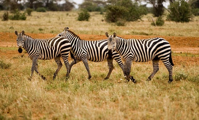
Photograph of Three Zebras
Taken by Boegh, some rights reserved.
Download the photograph and place it in your current working directory with the filename ‘zebra.jpg‘.
Making a prediction is straightforward, although interpreting the prediction requires some work.
The first step is to load the YOLOv3 Keras model. This might be the slowest part of making a prediction.
# load yolov3 model
model = load_model('model.h5')
Next, we need to load our new photograph and prepare it as suitable input to the model. The model expects inputs to be color images with the square shape of 416×416 pixels.
We can use the load_img() Keras function to load the image and the target_size argument to resize the image after loading. We can also use the img_to_array() function to convert the loaded PIL image object into a NumPy array, and then rescale the pixel values from 0-255 to 0-1 32-bit floating point values.
# load the image with the required size
image = load_img('zebra.jpg', target_size=(416, 416))
# convert to numpy array
image = img_to_array(image)
# scale pixel values to [0, 1]
image = image.astype('float32')
image /= 255.0
We will want to show the original photo again later, which means we will need to scale the bounding boxes of all detected objects from the square shape back to the original shape. As such, we can load the image and retrieve the original shape.
# load the image to get its shape
image = load_img('zebra.jpg')
width, height = image.size
We can tie all of this together into a convenience function named load_image_pixels() that takes the filename and target size and returns the scaled pixel data ready to provide as input to the Keras model, as well as the original width and height of the image.
# load and prepare an image
def load_image_pixels(filename, shape):
    # load the image to get its shape
    image = load_img(filename)
    width, height = image.size
    # load the image with the required size
    image = load_img(filename, target_size=shape)
    # convert to numpy array
    image = img_to_array(image)
    # scale pixel values to [0, 1]
    image = image.astype('float32')
    image /= 255.0
    # add a dimension so that we have one sample
    image = expand_dims(image, 0)
    return image, width, height
We can then call this function to load our photo of zebras.
# define the expected input shape for the model
input_w, input_h = 416, 416
# define our new photo
photo_filename = 'zebra.jpg'
# load and prepare image
image, image_w, image_h = load_image_pixels(photo_filename, (input_w, input_h))
We can now feed the photo into the Keras model and make a prediction.
# make prediction
yhat = model.predict(image)
# summarize the shape of the list of arrays
print([a.shape for a in yhat])
That’s it, at least for making a prediction. The complete example is listed below.
# load yolov3 model and perform object detection
# based on https://github.com/experiencor/keras-yolo3
from numpy import expand_dims
from keras.models import load_model
from keras.preprocessing.image import load_img
from keras.preprocessing.image import img_to_array

# load and prepare an image
def load_image_pixels(filename, shape):
    # load the image to get its shape
    image = load_img(filename)
    width, height = image.size
    # load the image with the required size
    image = load_img(filename, target_size=shape)
    # convert to numpy array
    image = img_to_array(image)
    # scale pixel values to [0, 1]
    image = image.astype('float32')
    image /= 255.0
    # add a dimension so that we have one sample
    image = expand_dims(image, 0)
    return image, width, height

# load yolov3 model
model = load_model('model.h5')
# define the expected input shape for the model
input_w, input_h = 416, 416
# define our new photo
photo_filename = 'zebra.jpg'
# load and prepare image
image, image_w, image_h = load_image_pixels(photo_filename, (input_w, input_h))
# make prediction
yhat = model.predict(image)
# summarize the shape of the list of arrays
print([a.shape for a in yhat])
Running the example returns a list of three NumPy arrays, the shape of which is displayed as output.
These arrays predict both the bounding boxes and class labels but are encoded. They must be interpreted.
[(1, 13, 13, 255), (1, 26, 26, 255), (1, 52, 52, 255)]
Make a Prediction and Interpret Result
The output of the model is, in fact, encoded candidate bounding boxes from three different grid sizes, and the boxes are defined the context of anchor boxes, carefully chosen based on an analysis of the size of objects in the MSCOCO dataset.
The script provided by experiencor provides a function called decode_netout() that will take each one of the NumPy arrays, one at a time, and decode the candidate bounding boxes and class predictions. Further, any bounding boxes that don’t confidently describe an object (e.g. all class probabilities are below a threshold) are ignored. We will use a probability of 60% or 0.6. The function returns a list of BoundBox instances that define the corners of each bounding box in the context of the input image shape and class probabilities.
# define the anchors
anchors = [[116,90, 156,198, 373,326], [30,61, 62,45, 59,119], [10,13, 16,30, 33,23]]
# define the probability threshold for detected objects
class_threshold = 0.6
boxes = list()
for i in range(len(yhat)):
	# decode the output of the network
	boxes += decode_netout(yhat[i][0], anchors[i], class_threshold, input_h, input_w)
Next, the bounding boxes can be stretched back into the shape of the original image. This is helpful as it means that later we can plot the original image and draw the bounding boxes, hopefully detecting real objects.
The experiencor script provides the correct_yolo_boxes() function to perform this translation of bounding box coordinates, taking the list of bounding boxes, the original shape of our loaded photograph, and the shape of the input to the network as arguments. The coordinates of the bounding boxes are updated directly.
# correct the sizes of the bounding boxes for the shape of the image
correct_yolo_boxes(boxes, image_h, image_w, input_h, input_w)
The model has predicted a lot of candidate bounding boxes, and most of the boxes will be referring to the same objects. The list of bounding boxes can be filtered and those boxes that overlap and refer to the same object can be merged. We can define the amount of overlap as a configuration parameter, in this case, 50% or 0.5. This filtering of bounding box regions is generally referred to as non-maximal suppression and is a required post-processing step.
The experiencor script provides this via the do_nms() function that takes the list of bounding boxes and a threshold parameter. Rather than purging the overlapping boxes, their predicted probability for their overlapping class is cleared. This allows the boxes to remain and be used if they also detect another object type.
# suppress non-maximal boxes
do_nms(boxes, 0.5)
This will leave us with the same number of boxes, but only very few of interest. We can retrieve just those boxes that strongly predict the presence of an object: that is are more than 60% confident. This can be achieved by enumerating over all boxes and checking the class prediction values. We can then look up the corresponding class label for the box and add it to the list. Each box must be considered for each class label, just in case the same box strongly predicts more than one object.
We can develop a get_boxes() function that does this and takes the list of boxes, known labels, and our classification threshold as arguments and returns parallel lists of boxes, labels, and scores.
# get all of the results above a threshold
def get_boxes(boxes, labels, thresh):
	v_boxes, v_labels, v_scores = list(), list(), list()
	# enumerate all boxes
	for box in boxes:
		# enumerate all possible labels
		for i in range(len(labels)):
			# check if the threshold for this label is high enough
			if box.classes[i] > thresh:
				v_boxes.append(box)
				v_labels.append(labels[i])
				v_scores.append(box.classes[i]*100)
				# don't break, many labels may trigger for one box
	return v_boxes, v_labels, v_scores
We can call this function with our list of boxes.
We also need a list of strings containing the class labels known to the model in the correct order used during training, specifically those class labels from the MSCOCO dataset. Thankfully, this is provided in the experiencor script.
# define the labels
labels = ["person", "bicycle", "car", "motorbike", "aeroplane", "bus", "train", "truck",
    "boat", "traffic light", "fire hydrant", "stop sign", "parking meter", "bench",
    "bird", "cat", "dog", "horse", "sheep", "cow", "elephant", "bear", "zebra", "giraffe",
    "backpack", "umbrella", "handbag", "tie", "suitcase", "frisbee", "skis", "snowboard",
    "sports ball", "kite", "baseball bat", "baseball glove", "skateboard", "surfboard",
    "tennis racket", "bottle", "wine glass", "cup", "fork", "knife", "spoon", "bowl", "banana",
    "apple", "sandwich", "orange", "broccoli", "carrot", "hot dog", "pizza", "donut", "cake",
    "chair", "sofa", "pottedplant", "bed", "diningtable", "toilet", "tvmonitor", "laptop", "mouse",
    "remote", "keyboard", "cell phone", "microwave", "oven", "toaster", "sink", "refrigerator",
    "book", "clock", "vase", "scissors", "teddy bear", "hair drier", "toothbrush"]
# get the details of the detected objects
v_boxes, v_labels, v_scores = get_boxes(boxes, labels, class_threshold)
Now that we have those few boxes of strongly predicted objects, we can summarize them.
# summarize what we found
for i in range(len(v_boxes)):
    print(v_labels[i], v_scores[i])
We can also plot our original photograph and draw the bounding box around each detected object. This can be achieved by retrieving the coordinates from each bounding box and creating a Rectangle object.
box = v_boxes[i]
# get coordinates
y1, x1, y2, x2 = box.ymin, box.xmin, box.ymax, box.xmax
# calculate width and height of the box
width, height = x2 - x1, y2 - y1
# create the shape
rect = Rectangle((x1, y1), width, height, fill=False, color='white')
# draw the box
ax.add_patch(rect)
We can also draw a string with the class label and confidence.
# draw text and score in top left corner
label = "%s (%.3f)" % (v_labels[i], v_scores[i])
pyplot.text(x1, y1, label, color='white')
The draw_boxes() function below implements this, taking the filename of the original photograph and the parallel lists of bounding boxes, labels and scores, and creates a plot showing all detected objects.
# draw all results
def draw_boxes(filename, v_boxes, v_labels, v_scores):
	# load the image
	data = pyplot.imread(filename)
	# plot the image
	pyplot.imshow(data)
	# get the context for drawing boxes
	ax = pyplot.gca()
	# plot each box
	for i in range(len(v_boxes)):
		box = v_boxes[i]
		# get coordinates
		y1, x1, y2, x2 = box.ymin, box.xmin, box.ymax, box.xmax
		# calculate width and height of the box
		width, height = x2 - x1, y2 - y1
		# create the shape
		rect = Rectangle((x1, y1), width, height, fill=False, color='white')
		# draw the box
		ax.add_patch(rect)
		# draw text and score in top left corner
		label = "%s (%.3f)" % (v_labels[i], v_scores[i])
		pyplot.text(x1, y1, label, color='white')
	# show the plot
	pyplot.show()
We can then call this function to plot our final result.
# draw what we found
draw_boxes(photo_filename, v_boxes, v_labels, v_scores)
We now have all of the elements required to make a prediction using the YOLOv3 model, interpret the results, and plot them for review.
The full code listing, including the original and modified functions taken from the experiencor script, are listed below for completeness.
# load yolov3 model and perform object detection
# based on https://github.com/experiencor/keras-yolo3
import numpy as np
from numpy import expand_dims
from keras.models import load_model
from keras.preprocessing.image import load_img
from keras.preprocessing.image import img_to_array
from matplotlib import pyplot
from matplotlib.patches import Rectangle

class BoundBox:
	def __init__(self, xmin, ymin, xmax, ymax, objness = None, classes = None):
		self.xmin = xmin
		self.ymin = ymin
		self.xmax = xmax
		self.ymax = ymax
		self.objness = objness
		self.classes = classes
		self.label = -1
		self.score = -1

	def get_label(self):
		if self.label == -1:
			self.label = np.argmax(self.classes)

		return self.label

	def get_score(self):
		if self.score == -1:
			self.score = self.classes[self.get_label()]

		return self.score

def _sigmoid(x):
	return 1. / (1. + np.exp(-x))

def decode_netout(netout, anchors, obj_thresh, net_h, net_w):
	grid_h, grid_w = netout.shape[:2]
	nb_box = 3
	netout = netout.reshape((grid_h, grid_w, nb_box, -1))
	nb_class = netout.shape[-1] - 5
	boxes = []
	netout[..., :2]  = _sigmoid(netout[..., :2])
	netout[..., 4:]  = _sigmoid(netout[..., 4:])
	netout[..., 5:]  = netout[..., 4][..., np.newaxis] * netout[..., 5:]
	netout[..., 5:] *= netout[..., 5:] > obj_thresh

	for i in range(grid_h*grid_w):
		row = i / grid_w
		col = i % grid_w
		for b in range(nb_box):
			# 4th element is objectness score
			objectness = netout[int(row)][int(col)][b][4]
			if(objectness.all() <= obj_thresh): continue
			# first 4 elements are x, y, w, and h
			x, y, w, h = netout[int(row)][int(col)][b][:4]
			x = (col + x) / grid_w # center position, unit: image width
			y = (row + y) / grid_h # center position, unit: image height
			w = anchors[2 * b + 0] * np.exp(w) / net_w # unit: image width
			h = anchors[2 * b + 1] * np.exp(h) / net_h # unit: image height
			# last elements are class probabilities
			classes = netout[int(row)][col][b][5:]
			box = BoundBox(x-w/2, y-h/2, x+w/2, y+h/2, objectness, classes)
			boxes.append(box)
	return boxes

def correct_yolo_boxes(boxes, image_h, image_w, net_h, net_w):
	new_w, new_h = net_w, net_h
	for i in range(len(boxes)):
		x_offset, x_scale = (net_w - new_w)/2./net_w, float(new_w)/net_w
		y_offset, y_scale = (net_h - new_h)/2./net_h, float(new_h)/net_h
		boxes[i].xmin = int((boxes[i].xmin - x_offset) / x_scale * image_w)
		boxes[i].xmax = int((boxes[i].xmax - x_offset) / x_scale * image_w)
		boxes[i].ymin = int((boxes[i].ymin - y_offset) / y_scale * image_h)
		boxes[i].ymax = int((boxes[i].ymax - y_offset) / y_scale * image_h)

def _interval_overlap(interval_a, interval_b):
	x1, x2 = interval_a
	x3, x4 = interval_b
	if x3 < x1:
		if x4 < x1:
			return 0
		else:
			return min(x2,x4) - x1
	else:
		if x2 < x3:
			 return 0
		else:
			return min(x2,x4) - x3

def bbox_iou(box1, box2):
	intersect_w = _interval_overlap([box1.xmin, box1.xmax], [box2.xmin, box2.xmax])
	intersect_h = _interval_overlap([box1.ymin, box1.ymax], [box2.ymin, box2.ymax])
	intersect = intersect_w * intersect_h
	w1, h1 = box1.xmax-box1.xmin, box1.ymax-box1.ymin
	w2, h2 = box2.xmax-box2.xmin, box2.ymax-box2.ymin
	union = w1*h1 + w2*h2 - intersect
	return float(intersect) / union

def do_nms(boxes, nms_thresh):
	if len(boxes) > 0:
		nb_class = len(boxes[0].classes)
	else:
		return
	for c in range(nb_class):
		sorted_indices = np.argsort([-box.classes[c] for box in boxes])
		for i in range(len(sorted_indices)):
			index_i = sorted_indices[i]
			if boxes[index_i].classes[c] == 0: continue
			for j in range(i+1, len(sorted_indices)):
				index_j = sorted_indices[j]
				if bbox_iou(boxes[index_i], boxes[index_j]) >= nms_thresh:
					boxes[index_j].classes[c] = 0

# load and prepare an image
def load_image_pixels(filename, shape):
	# load the image to get its shape
	image = load_img(filename)
	width, height = image.size
	# load the image with the required size
	image = load_img(filename, target_size=shape)
	# convert to numpy array
	image = img_to_array(image)
	# scale pixel values to [0, 1]
	image = image.astype('float32')
	image /= 255.0
	# add a dimension so that we have one sample
	image = expand_dims(image, 0)
	return image, width, height

# get all of the results above a threshold
def get_boxes(boxes, labels, thresh):
	v_boxes, v_labels, v_scores = list(), list(), list()
	# enumerate all boxes
	for box in boxes:
		# enumerate all possible labels
		for i in range(len(labels)):
			# check if the threshold for this label is high enough
			if box.classes[i] > thresh:
				v_boxes.append(box)
				v_labels.append(labels[i])
				v_scores.append(box.classes[i]*100)
				# don't break, many labels may trigger for one box
	return v_boxes, v_labels, v_scores

# draw all results
def draw_boxes(filename, v_boxes, v_labels, v_scores):
	# load the image
	data = pyplot.imread(filename)
	# plot the image
	pyplot.imshow(data)
	# get the context for drawing boxes
	ax = pyplot.gca()
	# plot each box
	for i in range(len(v_boxes)):
		box = v_boxes[i]
		# get coordinates
		y1, x1, y2, x2 = box.ymin, box.xmin, box.ymax, box.xmax
		# calculate width and height of the box
		width, height = x2 - x1, y2 - y1
		# create the shape
		rect = Rectangle((x1, y1), width, height, fill=False, color='white')
		# draw the box
		ax.add_patch(rect)
		# draw text and score in top left corner
		label = "%s (%.3f)" % (v_labels[i], v_scores[i])
		pyplot.text(x1, y1, label, color='white')
	# show the plot
	pyplot.show()

# load yolov3 model
model = load_model('model.h5')
# define the expected input shape for the model
input_w, input_h = 416, 416
# define our new photo
photo_filename = 'zebra.jpg'
# load and prepare image
image, image_w, image_h = load_image_pixels(photo_filename, (input_w, input_h))
# make prediction
yhat = model.predict(image)
# summarize the shape of the list of arrays
print([a.shape for a in yhat])
# define the anchors
anchors = [[116,90, 156,198, 373,326], [30,61, 62,45, 59,119], [10,13, 16,30, 33,23]]
# define the probability threshold for detected objects
class_threshold = 0.6
boxes = list()
for i in range(len(yhat)):
	# decode the output of the network
	boxes += decode_netout(yhat[i][0], anchors[i], class_threshold, input_h, input_w)
# correct the sizes of the bounding boxes for the shape of the image
correct_yolo_boxes(boxes, image_h, image_w, input_h, input_w)
# suppress non-maximal boxes
do_nms(boxes, 0.5)
# define the labels
labels = ["person", "bicycle", "car", "motorbike", "aeroplane", "bus", "train", "truck",
	"boat", "traffic light", "fire hydrant", "stop sign", "parking meter", "bench",
	"bird", "cat", "dog", "horse", "sheep", "cow", "elephant", "bear", "zebra", "giraffe",
	"backpack", "umbrella", "handbag", "tie", "suitcase", "frisbee", "skis", "snowboard",
	"sports ball", "kite", "baseball bat", "baseball glove", "skateboard", "surfboard",
	"tennis racket", "bottle", "wine glass", "cup", "fork", "knife", "spoon", "bowl", "banana",
	"apple", "sandwich", "orange", "broccoli", "carrot", "hot dog", "pizza", "donut", "cake",
	"chair", "sofa", "pottedplant", "bed", "diningtable", "toilet", "tvmonitor", "laptop", "mouse",
	"remote", "keyboard", "cell phone", "microwave", "oven", "toaster", "sink", "refrigerator",
	"book", "clock", "vase", "scissors", "teddy bear", "hair drier", "toothbrush"]
# get the details of the detected objects
v_boxes, v_labels, v_scores = get_boxes(boxes, labels, class_threshold)
# summarize what we found
for i in range(len(v_boxes)):
	print(v_labels[i], v_scores[i])
# draw what we found
draw_boxes(photo_filename, v_boxes, v_labels, v_scores)
Running the example again prints the shape of the raw output from the model.
This is followed by a summary of the objects detected by the model and their confidence. We can see that the model has detected three zebra, all above 90% likelihood.
[(1, 13, 13, 255), (1, 26, 26, 255), (1, 52, 52, 255)]
zebra 94.91060376167297
zebra 99.86329674720764
zebra 96.8708872795105
A plot of the photograph is created and the three bounding boxes are plotted. We can see that the model has indeed successfully detected the three zebra in the photograph.
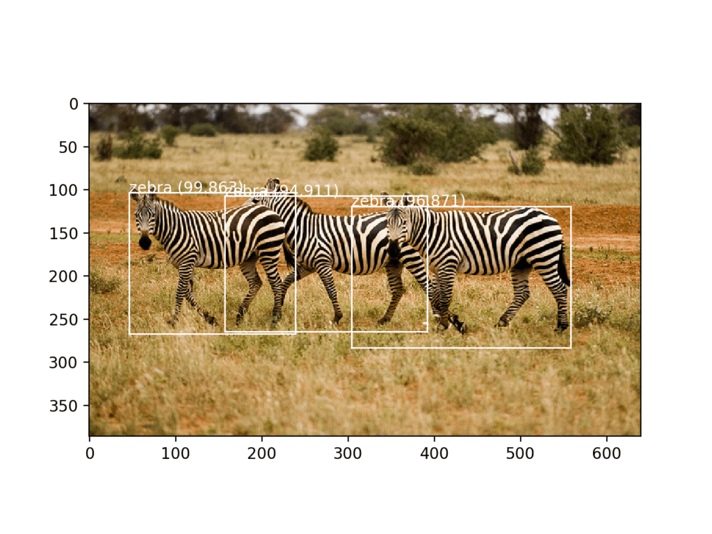
Photograph of Three Zebra Each Detected with the YOLOv3 Model and Localized with Bounding Boxes
Further Reading
This section provides more resources on the topic if you are looking to go deeper.
Papers
- You Only Look Once: Unified, Real-Time Object Detection, 2015.
- YOLO9000: Better, Faster, Stronger, 2016.
- YOLOv3: An Incremental Improvement, 2018.
API
Resources
- YOLO: Real-Time Object Detection, Homepage.
- Official DarkNet and YOLO Source Code, GitHub.
- Official YOLO: Real Time Object Detection.
- Huynh Ngoc Anh, experiencor, Home Page.
- experiencor/keras-yolo3, GitHub.
Other YOLO for Keras Projects
Summary
In this tutorial, you discovered how to develop a YOLOv3 model for object detection on new photographs.
Specifically, you learned:
- YOLO-based Convolutional Neural Network family of models for object detection and the most recent variation called YOLOv3.
- The best-of-breed open source library implementation of the YOLOv3 for the Keras deep learning library.
- How to use a pre-trained YOLOv3 to perform object localization and detection on new photographs.
Do you have any questions?
Ask your questions in the comments below and I will do my best to answer.
The post How to Perform Object Detection With YOLOv3 in Keras appeared first on Machine Learning Mastery.