Object detection is a challenging computer vision task that involves predicting both where the objects are in the image and what type of objects were detected.
The Mask Region-based Convolutional Neural Network, or Mask R-CNN, model is one of the state-of-the-art approaches for object recognition tasks. The Matterport Mask R-CNN project provides a library that allows you to develop and train Mask R-CNN Keras models for your own object detection tasks. Using the library can be tricky for beginners and requires the careful preparation of the dataset, although it allows fast training via transfer learning with top performing models trained on challenging object detection tasks, such as MS COCO.
In this tutorial, you will discover how to develop a Mask R-CNN model for kangaroo object detection in photographs.
After completing this tutorial, you will know:
How to prepare an object detection dataset ready for modeling with an R-CNN.
How to use transfer learning to train an object detection model on a new dataset.
How to evaluate a fit Mask R-CNN model on a test dataset and make predictions on new photos.
Let’s get started.
How to Train an Object Detection Model to Find Kangaroos in Photographs (R-CNN with Keras) Photo by Ronnie Robertson, some rights reserved.
Tutorial Overview
This tutorial is divided into five parts; they are:
How to Install Mask R-CNN for Keras
How to Prepare a Dataset for Object Detection
How to a Train Mask R-CNN Model for Kangaroo Detection
How to Evaluate a Mask R-CNN Model
How to Detect Kangaroos in New Photos
How to Install Mask R-CNN for Keras
Object detection is a task in computer vision that involves identifying the presence, location, and type of one or more objects in a given image.
It is a challenging problem that involves building upon methods for object recognition (e.g. where are they), object localization (e.g. what are their extent), and object classification (e.g. what are they).
The Region-Based Convolutional Neural Network, or R-CNN, is a family of convolutional neural network models designed for object detection, developed by Ross Girshick, et al. There are perhaps four main variations of the approach, resulting in the current pinnacle called Mask R-CNN. The Mask R-CNN introduced in the 2018 paper titled “Mask R-CNN” is the most recent variation of the family of models and supports both object detection and object segmentation. Object segmentation not only involves localizing objects in the image but also specifies a mask for the image, indicating exactly which pixels in the image belong to the object.
Mask R-CNN is a sophisticated model to implement, especially as compared to a simple or even state-of-the-art deep convolutional neural network model. Instead of developing an implementation of the R-CNN or Mask R-CNN model from scratch, we can use a reliable third-party implementation built on top of the Keras deep learning framework.
The best-of-breed third-party implementations of Mask R-CNN is the Mask R-CNN Project developed by Matterport. The project is open source released under a permissive license (e.g. MIT license) and the code has been widely used on a variety of projects and Kaggle competitions.
The first step is to install the library.
At the time of writing, there is no distributed version of the library, so we have to install it manually. The good news is that this is very easy.
Installation involves cloning the GitHub repository and running the installation script on your workstation. If you are having trouble, see the installation instructions buried in the library’s readme file.
Want Results with Deep Learning for Computer Vision?
Take my free 7-day email crash course now (with sample code).
Click to sign-up and also get a free PDF Ebook version of the course.
Change directory into the Mask_RCNN directory and run the installation script.
From the command line, type the following:
cd Mask_RCNN
python setup.py install
On Linux or MacOS, you may need to install the software with sudo permissions; for example, you may see an error such as:
error: can't create or remove files in install directory
In that case, install the software with sudo:
sudo python setup.py install
If you are using a Python virtual environment (virtualenv), such as on an EC2 Deep Learning AMI instance (recommended for this tutorial), you can install Mask_RCNN into your environment as follows:
The library will then install directly and you will see a lot of successful installation messages ending with the following:
...
Finished processing dependencies for mask-rcnn==2.1
This confirms that you installed the library successfully and that you have the latest version, which at the time of writing is version 2.1.
Step 3: Confirm the Library Was Installed
It is always a good idea to confirm that the library was installed correctly.
You can confirm that the library was installed correctly by querying it via the pip command; for example:
pip show mask-rcnn
You should see output informing you of the version and installation location; for example:
Name: mask-rcnn
Version: 2.1
Summary: Mask R-CNN for object detection and instance segmentation
Home-page: https://github.com/matterport/Mask_RCNN
Author: Matterport
Author-email: waleed.abdulla@gmail.com
License: MIT
Location: ...
Requires:
Required-by:
We are now ready to use the library.
How to Prepare a Dataset for Object Detection
Next, we need a dataset to model.
In this tutorial, we will use the kangaroo dataset, made available by Huynh Ngoc Anh (experiencor). The dataset is comprised of 183 photographs that contain kangaroos, and XML annotation files that provide bounding boxes for the kangaroos in each photograph.
The Mask R-CNN is designed to learn to predict both bounding boxes for objects as well as masks for those detected objects, and the kangaroo dataset does not provide masks. As such, we will use the dataset to learn a kangaroo object detection task, and ignore the masks and not focus on the image segmentation capabilities of the model.
There are a few steps required in order to prepare this dataset for modeling and we will work through each in turn in this section, including downloading the dataset, parsing the annotations file, developing a KangarooDataset object that can be used by the Mask_RCNN library, then testing the dataset object to confirm that we are loading images and annotations correctly.
Install Dataset
The first step is to download the dataset into your current working directory.
This can be achieved by cloning the GitHub repository directly, as follows:
This will create a new directory called “kangaroo” with a subdirectory called ‘images/‘ that contains all of the JPEG photos of kangaroos and a subdirectory called ‘annotes/‘ that contains all of the XML files that describe the locations of kangaroos in each photo.
kangaroo
├── annots
└── images
Looking in each subdirectory, you can see that the photos and annotation files use a consistent naming convention, with filenames using a 5-digit zero-padded numbering system; for example:
This makes matching photographs and annotation files together very easy.
We can also see that the numbering system is not contiguous, that there are some photos missing, e.g. there is no ‘00007‘ JPG or XML.
This means that we should focus on loading the list of actual files in the directory rather than using a numbering system.
Parse Annotation File
The next step is to figure out how to load the annotation files.
First, open the first annotation file (annots/00001.xml) and take a look; you should see:
Kangaroo00001.jpg...Unknown45031930
We can see that the annotation file contains a “size” element that describes the shape of the photograph, and one or more “object” elements that describe the bounding boxes for the kangaroo objects in the photograph.
The size and the bounding boxes are the minimum information that we require from each annotation file. We could write some careful XML parsing code to process these annotation files, and that would be a good idea for a production system. Instead, we will short-cut development and use XPath queries to directly extract the data that we need from each file, e.g. a //size query to extract the size element and a //object or a //bndbox query to extract the bounding box elements.
Python provides the ElementTree API that can be used to load and parse an XML file and we can use the find() and findall() functions to perform the XPath queries on a loaded document.
First, the annotation file must be loaded and parsed as an ElementTree object.
# load and parse the file
tree = ElementTree.parse(filename)
Once loaded, we can retrieve the root element of the document from which we can perform our XPath queries.
# get the root of the document
root = tree.getroot()
We can use the findall() function with a query for ‘.//bndbox‘ to find all ‘bndbox‘ elements, then enumerate each to extract the x and y,min and max values that define each bounding box.
The element text can also be parsed to integer values.
# extract each bounding box
for box in root.findall('.//bndbox'):
	xmin = int(box.find('xmin').text)
	ymin = int(box.find('ymin').text)
	xmax = int(box.find('xmax').text)
	ymax = int(box.find('ymax').text)
	coors = [xmin, ymin, xmax, ymax]
We can then collect the definition of each bounding box into a list.
The dimensions of the image may also be helpful, which can be queried directly.
We can tie all of this together into a function that will take the annotation filename as an argument, extract the bounding box and image dimension details, and return them for use.
The extract_boxes() function below implements this behavior.
# function to extract bounding boxes from an annotation file
def extract_boxes(filename):
# load and parse the file
tree = ElementTree.parse(filename)
# get the root of the document
root = tree.getroot()
# extract each bounding box
boxes = list()
for box in root.findall('.//bndbox'):
xmin = int(box.find('xmin').text)
ymin = int(box.find('ymin').text)
xmax = int(box.find('xmax').text)
ymax = int(box.find('ymax').text)
coors = [xmin, ymin, xmax, ymax]
boxes.append(coors)
# extract image dimensions
width = int(root.find('.//size/width').text)
height = int(root.find('.//size/height').text)
return boxes, width, height
We can test out this function on our annotation files, for example, on the first annotation file in the directory.
The complete example is listed below.
# example of extracting bounding boxes from an annotation file
from xml.etree import ElementTree
# function to extract bounding boxes from an annotation file
def extract_boxes(filename):
	# load and parse the file
	tree = ElementTree.parse(filename)
	# get the root of the document
	root = tree.getroot()
	# extract each bounding box
	boxes = list()
	for box in root.findall('.//bndbox'):
		xmin = int(box.find('xmin').text)
		ymin = int(box.find('ymin').text)
		xmax = int(box.find('xmax').text)
		ymax = int(box.find('ymax').text)
		coors = [xmin, ymin, xmax, ymax]
		boxes.append(coors)
	# extract image dimensions
	width = int(root.find('.//size/width').text)
	height = int(root.find('.//size/height').text)
	return boxes, width, height
# extract details form annotation file
boxes, w, h = extract_boxes('kangaroo/annots/00001.xml')
# summarize extracted details
print(boxes, w, h)
Running the example returns a list that contains the details of each bounding box in the annotation file, as well as two integers for the width and height of the photograph.
Now that we know how to load the annotation file, we can look at using this functionality to develop a Dataset object.
Develop KangarooDataset Object
The mask-rcnn library requires that train, validation, and test datasets be managed by a mrcnn.utils.Dataset object.
This means that a new class must be defined that extends the mrcnn.utils.Dataset class and defines a function to load the dataset, with any name you like such as load_dataset(), and override two functions, one for loading a mask called load_mask() and one for loading an image reference (path or URL) called image_reference().
# class that defines and loads the kangaroo dataset
class KangarooDataset(Dataset):
	# load the dataset definitions
	def load_dataset(self, dataset_dir, is_train=True):
		# ...

	# load the masks for an image
	def load_mask(self, image_id):
		# ...

	# load an image reference
	def image_reference(self, image_id):
		# ...
To use a Dataset object, it is instantiated, then your custom load function must be called, then finally the built-in prepare() function is called.
For example, we will create a new class called KangarooDataset that will be used as follows:
# prepare the dataset
train_set = KangarooDataset()
train_set.load_dataset(...)
train_set.prepare()
The custom load function, e.g. load_dataset() is responsible for both defining the classes and for defining the images in the dataset.
Classes are defined by calling the built-in add_class() function and specifying the ‘source‘ (the name of the dataset), the ‘class_id‘ or integer for the class (e.g. 1 for the first lass as 0 is reserved for the background class), and the ‘class_name‘ (e.g. ‘kangaroo‘).
# define one class
self.add_class("dataset", 1, "kangaroo")
Objects are defined by a call to the built-in add_image() function and specifying the ‘source‘ (the name of the dataset), a unique ‘image_id‘ (e.g. the filename without the file extension like ‘00001‘), and the path for where the image can be loaded (e.g. ‘kangaroo/images/00001.jpg‘).
This will define an “image info” dictionary for the image that can be retrieved later via the index or order in which the image was added to the dataset. You can also specify other arguments that will be added to the image info dictionary, such as an ‘annotation‘ to define the annotation path.
# add to dataset
self.add_image('dataset', image_id='00001', path='kangaroo/images/00001.jpg', annotation='kangaroo/annots/00001.xml')
For example, we can implement a load_dataset() function that takes the path to the dataset directory and loads all images in the dataset.
Note, testing revealed that there is an issue with image number ‘00090‘, so we will exclude it from the dataset.
# load the dataset definitions
def load_dataset(self, dataset_dir):
	# define one class
	self.add_class("dataset", 1, "kangaroo")
	# define data locations
	images_dir = dataset_dir + '/images/'
	annotations_dir = dataset_dir + '/annots/'
	# find all images
	for filename in listdir(images_dir):
		# extract image id
		image_id = filename[:-4]
		# skip bad images
		if image_id in ['00090']:
			continue
		img_path = images_dir + filename
		ann_path = annotations_dir + image_id + '.xml'
		# add to dataset
		self.add_image('dataset', image_id=image_id, path=img_path, annotation=ann_path)
We can go one step further and add one more argument to the function to define whether the Dataset instance is for training or test/validation. We have about 160 photos, so we can use about 20%, or the last 32 photos, as a test or validation dataset and the first 131, or 80%, as the training dataset.
This division can be made using the integer in the filename, where all photos before photo number 150 will be train and equal or after 150 used for test. The updated load_dataset() with support for train and test datasets is provided below.
# load the dataset definitions
def load_dataset(self, dataset_dir, is_train=True):
	# define one class
	self.add_class("dataset", 1, "kangaroo")
	# define data locations
	images_dir = dataset_dir + '/images/'
	annotations_dir = dataset_dir + '/annots/'
	# find all images
	for filename in listdir(images_dir):
		# extract image id
		image_id = filename[:-4]
		# skip bad images
		if image_id in ['00090']:
			continue
		# skip all images after 150 if we are building the train set
		if is_train and int(image_id) >= 150:
			continue
		# skip all images before 150 if we are building the test/val set
		if not is_train and int(image_id) < 150:
			continue
		img_path = images_dir + filename
		ann_path = annotations_dir + image_id + '.xml'
		# add to dataset
		self.add_image('dataset', image_id=image_id, path=img_path, annotation=ann_path)
Next, we need to define the load_mask() function for loading the mask for a given ‘image_id‘.
In this case, the ‘image_id‘ is the integer index for an image in the dataset, assigned based on the order that the image was added via a call to add_image() when loading the dataset. The function must return an array of one or more masks for the photo associated with the image_id, and the classes for each mask.
We don’t have masks, but we do have bounding boxes. We can load the bounding boxes for a given photo and return them as masks. The library will then infer bounding boxes from our “masks” which will be the same size.
First, we must load the annotation file for the image_id. This involves first retrieving the ‘image info‘ dict for the image_id, then retrieving the annotations path that we stored for the image via our prior call to add_image(). We can then use the path in our call to extract_boxes() developed in the previous section to get the list of bounding boxes and the dimensions of the image.
# get details of image
info = self.image_info[image_id]
# define box file location
path = info['annotation']
# load XML
boxes, w, h = self.extract_boxes(path)
We can now define a mask for each bounding box, and an associated class.
A mask is a two-dimensional array with the same dimensions as the photograph with all zero values where the object isn’t and all one values where the object is in the photograph.
We can achieve this by creating a NumPy array with all zero values for the known size of the image and one channel for each bounding box.
# create one array for all masks, each on a different channel
masks = zeros([h, w, len(boxes)], dtype='uint8')
Each bounding box is defined as min and max, x and y coordinates of the box.
These can be used directly to define row and column ranges in the array that can then be marked as 1.
# create masks
for i in range(len(boxes)):
	box = boxes[i]
	row_s, row_e = box[1], box[3]
	col_s, col_e = box[0], box[2]
	masks[row_s:row_e, col_s:col_e, i] = 1
All objects have the same class in this dataset. We can retrieve the class index via the ‘class_names‘ dictionary, then add it to a list to be returned alongside the masks.
self.class_names.index('kangaroo')
Tying this together, the complete load_mask() function is listed below.
# load the masks for an image
def load_mask(self, image_id):
	# get details of image
	info = self.image_info[image_id]
	# define box file location
	path = info['annotation']
	# load XML
	boxes, w, h = self.extract_boxes(path)
	# create one array for all masks, each on a different channel
	masks = zeros([h, w, len(boxes)], dtype='uint8')
	# create masks
	class_ids = list()
	for i in range(len(boxes)):
		box = boxes[i]
		row_s, row_e = box[1], box[3]
		col_s, col_e = box[0], box[2]
		masks[row_s:row_e, col_s:col_e, i] = 1
		class_ids.append(self.class_names.index('kangaroo'))
	return masks, asarray(class_ids, dtype='int32')
Finally, we must implement the image_reference() function.
This function is responsible for returning the path or URL for a given ‘image_id‘, which we know is just the ‘path‘ property on the ‘image info‘ dict.
# load an image reference
def image_reference(self, image_id):
	info = self.image_info[image_id]
	return info['path']
And that’s it. We have successfully defined a Dataset object for the mask-rcnn library for our Kangaroo dataset.
The complete listing of the class and creating a train and test dataset is provided below.
# split into train and test set
from os import listdir
from xml.etree import ElementTree
from numpy import zeros
from numpy import asarray
from mrcnn.utils import Dataset

# class that defines and loads the kangaroo dataset
class KangarooDataset(Dataset):
	# load the dataset definitions
	def load_dataset(self, dataset_dir, is_train=True):
		# define one class
		self.add_class("dataset", 1, "kangaroo")
		# define data locations
		images_dir = dataset_dir + '/images/'
		annotations_dir = dataset_dir + '/annots/'
		# find all images
		for filename in listdir(images_dir):
			# extract image id
			image_id = filename[:-4]
			# skip bad images
			if image_id in ['00090']:
				continue
			# skip all images after 150 if we are building the train set
			if is_train and int(image_id) >= 150:
				continue
			# skip all images before 150 if we are building the test/val set
			if not is_train and int(image_id) < 150:
				continue
			img_path = images_dir + filename
			ann_path = annotations_dir + image_id + '.xml'
			# add to dataset
			self.add_image('dataset', image_id=image_id, path=img_path, annotation=ann_path)

	# extract bounding boxes from an annotation file
	def extract_boxes(self, filename):
		# load and parse the file
		tree = ElementTree.parse(filename)
		# get the root of the document
		root = tree.getroot()
		# extract each bounding box
		boxes = list()
		for box in root.findall('.//bndbox'):
			xmin = int(box.find('xmin').text)
			ymin = int(box.find('ymin').text)
			xmax = int(box.find('xmax').text)
			ymax = int(box.find('ymax').text)
			coors = [xmin, ymin, xmax, ymax]
			boxes.append(coors)
		# extract image dimensions
		width = int(root.find('.//size/width').text)
		height = int(root.find('.//size/height').text)
		return boxes, width, height

	# load the masks for an image
	def load_mask(self, image_id):
		# get details of image
		info = self.image_info[image_id]
		# define box file location
		path = info['annotation']
		# load XML
		boxes, w, h = self.extract_boxes(path)
		# create one array for all masks, each on a different channel
		masks = zeros([h, w, len(boxes)], dtype='uint8')
		# create masks
		class_ids = list()
		for i in range(len(boxes)):
			box = boxes[i]
			row_s, row_e = box[1], box[3]
			col_s, col_e = box[0], box[2]
			masks[row_s:row_e, col_s:col_e, i] = 1
			class_ids.append(self.class_names.index('kangaroo'))
		return masks, asarray(class_ids, dtype='int32')

	# load an image reference
	def image_reference(self, image_id):
		info = self.image_info[image_id]
		return info['path']

# train set
train_set = KangarooDataset()
train_set.load_dataset('kangaroo', is_train=True)
train_set.prepare()
print('Train: %d' % len(train_set.image_ids))

# test/val set
test_set = KangarooDataset()
test_set.load_dataset('kangaroo', is_train=False)
test_set.prepare()
print('Test: %d' % len(test_set.image_ids))
Running the example successfully loads and prepares the train and test dataset and prints the number of images in each.
Train: 131
Test: 32
Now that we have defined the dataset, let’s confirm that the images, masks, and bounding boxes are handled correctly.
Test KangarooDataset Object
The first useful test is to confirm that the images and masks can be loaded correctly.
We can test this by creating a dataset and loading an image via a call to the load_image() function with an image_id, then load the mask for the image via a call to the load_mask() function with the same image_id.
Next, we can plot the photograph using the Matplotlib API, then plot the first mask over the top with an alpha value so that the photograph underneath can still be seen
# plot one photograph and mask
from os import listdir
from xml.etree import ElementTree
from numpy import zeros
from numpy import asarray
from mrcnn.utils import Dataset
from matplotlib import pyplot
# class that defines and loads the kangaroo dataset
class KangarooDataset(Dataset):
# load the dataset definitions
def load_dataset(self, dataset_dir, is_train=True):
# define one class
self.add_class("dataset", 1, "kangaroo")
# define data locations
images_dir = dataset_dir + '/images/'
annotations_dir = dataset_dir + '/annots/'
# find all images
for filename in listdir(images_dir):
# extract image id
image_id = filename[:-4]
# skip bad images
if image_id in ['00090']:
continue
# skip all images after 150 if we are building the train set
if is_train and int(image_id) >= 150:
continue
# skip all images before 150 if we are building the test/val set
if not is_train and int(image_id) < 150:
continue
img_path = images_dir + filename
ann_path = annotations_dir + image_id + '.xml'
# add to dataset
self.add_image('dataset', image_id=image_id, path=img_path, annotation=ann_path)
# extract bounding boxes from an annotation file
def extract_boxes(self, filename):
# load and parse the file
tree = ElementTree.parse(filename)
# get the root of the document
root = tree.getroot()
# extract each bounding box
boxes = list()
for box in root.findall('.//bndbox'):
xmin = int(box.find('xmin').text)
ymin = int(box.find('ymin').text)
xmax = int(box.find('xmax').text)
ymax = int(box.find('ymax').text)
coors = [xmin, ymin, xmax, ymax]
boxes.append(coors)
# extract image dimensions
width = int(root.find('.//size/width').text)
height = int(root.find('.//size/height').text)
return boxes, width, height
# load the masks for an image
def load_mask(self, image_id):
# get details of image
info = self.image_info[image_id]
# define box file location
path = info['annotation']
# load XML
boxes, w, h = self.extract_boxes(path)
# create one array for all masks, each on a different channel
masks = zeros([h, w, len(boxes)], dtype='uint8')
# create masks
class_ids = list()
for i in range(len(boxes)):
box = boxes[i]
row_s, row_e = box[1], box[3]
col_s, col_e = box[0], box[2]
masks[row_s:row_e, col_s:col_e, i] = 1
class_ids.append(self.class_names.index('kangaroo'))
return masks, asarray(class_ids, dtype='int32')
# load an image reference
def image_reference(self, image_id):
info = self.image_info[image_id]
return info['path']
# train set
train_set = KangarooDataset()
train_set.load_dataset('kangaroo', is_train=True)
train_set.prepare()
# load an image
image_id = 0
image = train_set.load_image(image_id)
print(image.shape)
# load image mask
mask, class_ids = train_set.load_mask(image_id)
print(mask.shape)
# plot image
pyplot.imshow(image)
# plot mask
pyplot.imshow(mask[:, :, 0], cmap='gray', alpha=0.5)
pyplot.show()
Running the example first prints the shape of the photograph and mask NumPy arrays.
We can confirm that both arrays have the same width and height and only differ in terms of the number of channels. We can also see that the first photograph (e.g. image_id=0) in this case only has one mask.
(626, 899, 3)
(626, 899, 1)
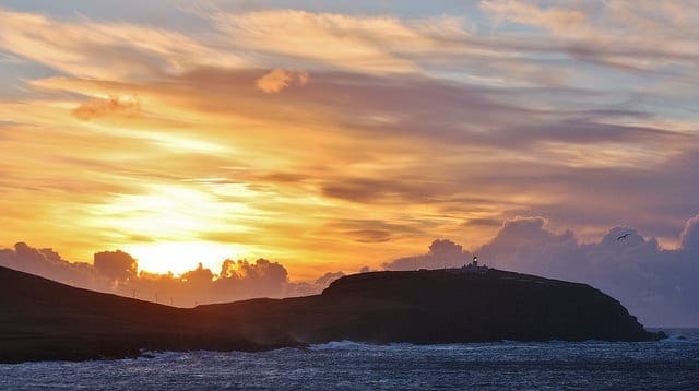
A plot of the photograph is also created with the first mask overlaid.
In this case, we can see that one kangaroo is present in the photo and that the mask correctly bounds the kangaroo.
Photograph of Kangaroo With Object Detection Mask Overlaid
We could repeat this for the first nine photos in the dataset, plotting each photo in one figure as a subplot and plotting all masks for each photo.
# plot first few images
for i in range(9):
	# define subplot
	pyplot.subplot(330 + 1 + i)
	# plot raw pixel data
	image = train_set.load_image(i)
	pyplot.imshow(image)
	# plot all masks
	mask, _ = train_set.load_mask(i)
	for j in range(mask.shape[2]):
		pyplot.imshow(mask[:, :, j], cmap='gray', alpha=0.3)
# show the figure
pyplot.show()
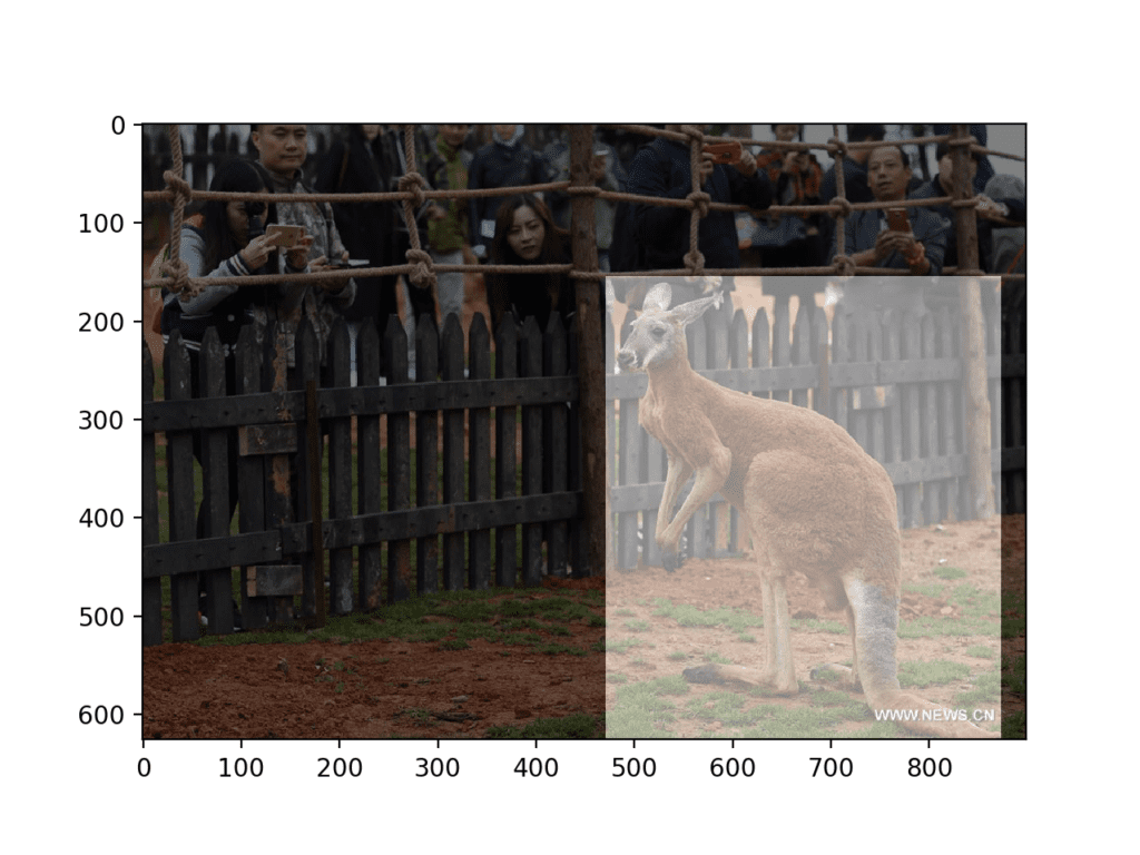
Running the example shows that photos are loaded correctly and that those photos with multiple objects correctly have separate masks defined.
Plot of First Nine Photos of Kangaroos in the Training Dataset With Object Detection Masks
Another useful debugging step might be to load all of the ‘image info‘ objects in the dataset and print them to the console.
This can help to confirm that all of the calls to the add_image() function in the load_dataset() function worked as expected.
# enumerate all images in the dataset
for image_id in train_set.image_ids:
	# load image info
	info = train_set.image_info[image_id]
	# display on the console
	print(info)
Running this code on the loaded training dataset will then show all of the ‘image info‘ dictionaries, showing the paths and ids for each image in the dataset.
Finally, the mask-rcnn library provides utilities for displaying images and masks. We can use some of these built-in functions to confirm that the Dataset is operating correctly.
For example, the mask-rcnn library provides the mrcnn.visualize.display_instances() function that will show a photograph with bounding boxes, masks, and class labels. This requires that the bounding boxes are extracted from the masks via the extract_bboxes() function.
# define image id
image_id = 1
# load the image
image = train_set.load_image(image_id)
# load the masks and the class ids
mask, class_ids = train_set.load_mask(image_id)
# extract bounding boxes from the masks
bbox = extract_bboxes(mask)
# display image with masks and bounding boxes
display_instances(image, bbox, mask, class_ids, train_set.class_names)
For completeness, the full code listing is provided below.
# display image with masks and bounding boxes
from os import listdir
from xml.etree import ElementTree
from numpy import zeros
from numpy import asarray
from mrcnn.utils import Dataset
from mrcnn.visualize import display_instances
from mrcnn.utils import extract_bboxes

# class that defines and loads the kangaroo dataset
class KangarooDataset(Dataset):
	# load the dataset definitions
	def load_dataset(self, dataset_dir, is_train=True):
		# define one class
		self.add_class("dataset", 1, "kangaroo")
		# define data locations
		images_dir = dataset_dir + '/images/'
		annotations_dir = dataset_dir + '/annots/'
		# find all images
		for filename in listdir(images_dir):
			# extract image id
			image_id = filename[:-4]
			# skip bad images
			if image_id in ['00090']:
				continue
			# skip all images after 150 if we are building the train set
			if is_train and int(image_id) >= 150:
				continue
			# skip all images before 150 if we are building the test/val set
			if not is_train and int(image_id) < 150:
				continue
			img_path = images_dir + filename
			ann_path = annotations_dir + image_id + '.xml'
			# add to dataset
			self.add_image('dataset', image_id=image_id, path=img_path, annotation=ann_path)

	# extract bounding boxes from an annotation file
	def extract_boxes(self, filename):
		# load and parse the file
		tree = ElementTree.parse(filename)
		# get the root of the document
		root = tree.getroot()
		# extract each bounding box
		boxes = list()
		for box in root.findall('.//bndbox'):
			xmin = int(box.find('xmin').text)
			ymin = int(box.find('ymin').text)
			xmax = int(box.find('xmax').text)
			ymax = int(box.find('ymax').text)
			coors = [xmin, ymin, xmax, ymax]
			boxes.append(coors)
		# extract image dimensions
		width = int(root.find('.//size/width').text)
		height = int(root.find('.//size/height').text)
		return boxes, width, height

	# load the masks for an image
	def load_mask(self, image_id):
		# get details of image
		info = self.image_info[image_id]
		# define box file location
		path = info['annotation']
		# load XML
		boxes, w, h = self.extract_boxes(path)
		# create one array for all masks, each on a different channel
		masks = zeros([h, w, len(boxes)], dtype='uint8')
		# create masks
		class_ids = list()
		for i in range(len(boxes)):
			box = boxes[i]
			row_s, row_e = box[1], box[3]
			col_s, col_e = box[0], box[2]
			masks[row_s:row_e, col_s:col_e, i] = 1
			class_ids.append(self.class_names.index('kangaroo'))
		return masks, asarray(class_ids, dtype='int32')

	# load an image reference
	def image_reference(self, image_id):
		info = self.image_info[image_id]
		return info['path']

# train set
train_set = KangarooDataset()
train_set.load_dataset('kangaroo', is_train=True)
train_set.prepare()
# define image id
image_id = 1
# load the image
image = train_set.load_image(image_id)
# load the masks and the class ids
mask, class_ids = train_set.load_mask(image_id)
# extract bounding boxes from the masks
bbox = extract_bboxes(mask)
# display image with masks and bounding boxes
display_instances(image, bbox, mask, class_ids, train_set.class_names)
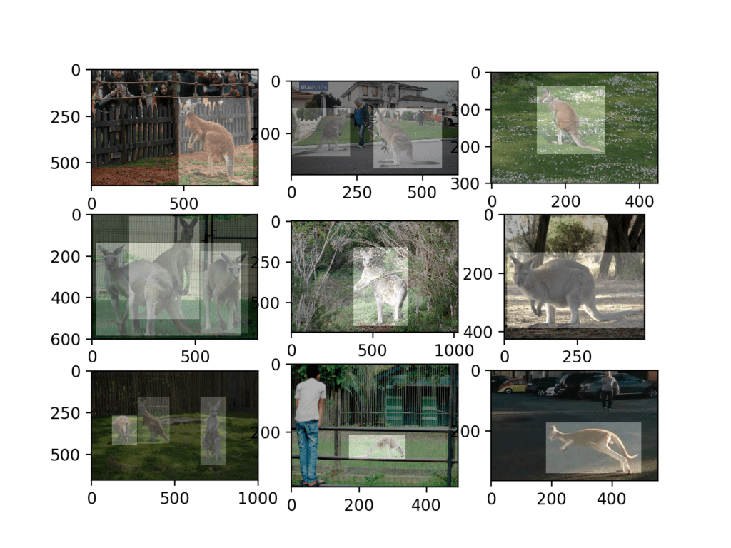
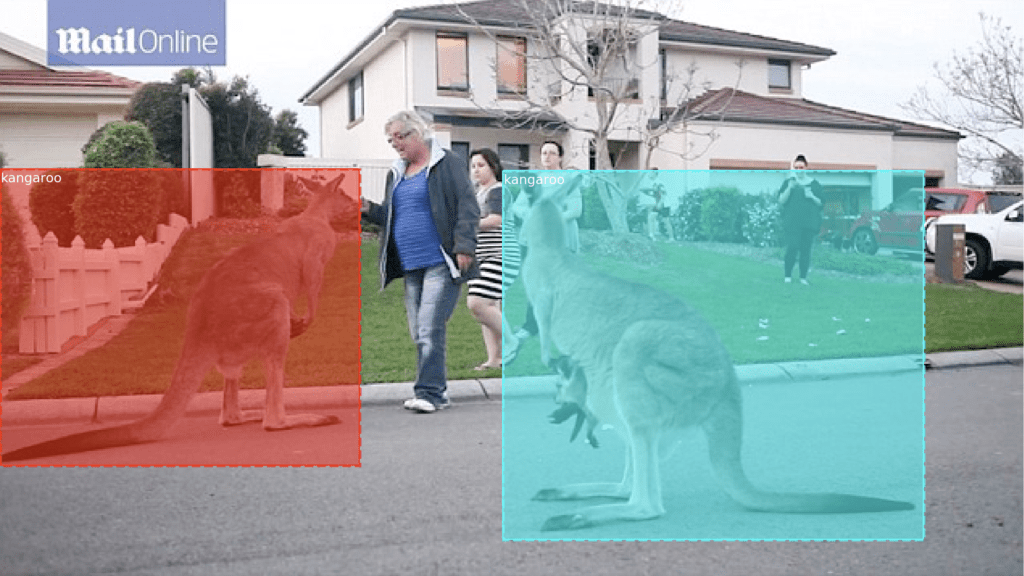
Running the example creates a plot showing the photograph with the mask for each object in a separate color.
The bounding boxes match the masks exactly, by design, and are shown with dotted outlines. Finally, each object is marked with the class label, which in this case is ‘kangaroo‘.
Photograph Showing Object Detection Masks, Bounding Boxes, and Class Labels
Now that we are confident that our dataset is being loaded correctly, we can use it to fit a Mask R-CNN model.
How to Train Mask R-CNN Model for Kangaroo Detection
A Mask R-CNN model can be fit from scratch, although like other computer vision applications, time can be saved and performance can be improved by using transfer learning.
The Mask R-CNN model pre-fit on the MS COCO object detection dataset can be used as a starting point and then tailored to the specific dataset, in this case, the kangaroo dataset.
The first step is to download the model file (architecture and weights) for the pre-fit Mask R-CNN model. The weights are available from the GitHub project and the file is about 250 megabytes.
Download the model weights to a file with the name ‘mask_rcnn_coco.h5‘ in your current working directory.
Next, a configuration object for the model must be defined.
This is a new class that extends the mrcnn.config.Config class and defines properties of both the prediction problem (such as name and the number of classes) and the algorithm for training the model (such as the learning rate).
The configuration must define the name of the configuration via the ‘NAME‘ attribute, e.g. ‘kangaroo_cfg‘, that will be used to save details and models to file during the run. The configuration must also define the number of classes in the prediction problem via the ‘NUM_CLASSES‘ attribute. In this case, we only have one object type of kangaroo, although there is always an additional class for the background.
Finally, we must define the number of samples (photos) used in each training epoch. This will be the number of photos in the training dataset, in this case, 131.
Tying this together, our custom KangarooConfig class is defined below.
# define a configuration for the model
class KangarooConfig(Config):
	# Give the configuration a recognizable name
	NAME = "kangaroo_cfg"
	# Number of classes (background + kangaroo)
	NUM_CLASSES = 1 + 1
	# Number of training steps per epoch
	STEPS_PER_EPOCH = 131

# prepare config
config = KangarooConfig()
Next, we can define our model.
This is achieved by creating an instance of the mrcnn.model.MaskRCNN class and specifying the model will be used for training via setting the ‘mode‘ argument to ‘training‘.
The ‘config‘ argument must also be specified with an instance of our KangarooConfig class.
Finally, a directory is needed where configuration files can be saved and where checkpoint models can be saved at the end of each epoch. We will use the current working directory.
# define the model
model = MaskRCNN(mode='training', model_dir='./', config=config)
Next, the pre-defined model architecture and weights can be loaded. This can be achieved by calling the load_weights() function on the model and specifying the path to the downloaded ‘mask_rcnn_coco.h5‘ file.
The model will be used as-is, although the class-specific output layers will be removed so that new output layers can be defined and trained. This can be done by specifying the ‘exclude‘ argument and listing all of the output layers to exclude or remove from the model after it is loaded. This includes the output layers for the classification label, bounding boxes, and masks.
Next, the model can be fit on the training dataset by calling the train() function and passing in both the training dataset and the validation dataset. We can also specify the learning rate as the default learning rate in the configuration (0.001).
We can also specify what layers to train. In this case, we will only train the heads, that is the output layers of the model.
We could follow this training with further epochs that fine-tune all of the weights in the model. This could be achieved by using a smaller learning rate and changing the ‘layer’ argument from ‘heads’ to ‘all’.
The complete example of training a Mask R-CNN on the kangaroo dataset is listed below.
This may take some time to execute on the CPU, even with modern hardware. I recommend running the code with a GPU, such as on Amazon EC2, where it will finish in about five minutes on a P3 type hardware.
# fit a mask rcnn on the kangaroo dataset
from os import listdir
from xml.etree import ElementTree
from numpy import zeros
from numpy import asarray
from mrcnn.utils import Dataset
from mrcnn.config import Config
from mrcnn.model import MaskRCNN
# class that defines and loads the kangaroo dataset
class KangarooDataset(Dataset):
# load the dataset definitions
def load_dataset(self, dataset_dir, is_train=True):
# define one class
self.add_class("dataset", 1, "kangaroo")
# define data locations
images_dir = dataset_dir + '/images/'
annotations_dir = dataset_dir + '/annots/'
# find all images
for filename in listdir(images_dir):
# extract image id
image_id = filename[:-4]
# skip bad images
if image_id in ['00090']:
continue
# skip all images after 150 if we are building the train set
if is_train and int(image_id) >= 150:
continue
# skip all images before 150 if we are building the test/val set
if not is_train and int(image_id) < 150:
continue
img_path = images_dir + filename
ann_path = annotations_dir + image_id + '.xml'
# add to dataset
self.add_image('dataset', image_id=image_id, path=img_path, annotation=ann_path)
# extract bounding boxes from an annotation file
def extract_boxes(self, filename):
# load and parse the file
tree = ElementTree.parse(filename)
# get the root of the document
root = tree.getroot()
# extract each bounding box
boxes = list()
for box in root.findall('.//bndbox'):
xmin = int(box.find('xmin').text)
ymin = int(box.find('ymin').text)
xmax = int(box.find('xmax').text)
ymax = int(box.find('ymax').text)
coors = [xmin, ymin, xmax, ymax]
boxes.append(coors)
# extract image dimensions
width = int(root.find('.//size/width').text)
height = int(root.find('.//size/height').text)
return boxes, width, height
# load the masks for an image
def load_mask(self, image_id):
# get details of image
info = self.image_info[image_id]
# define box file location
path = info['annotation']
# load XML
boxes, w, h = self.extract_boxes(path)
# create one array for all masks, each on a different channel
masks = zeros([h, w, len(boxes)], dtype='uint8')
# create masks
class_ids = list()
for i in range(len(boxes)):
box = boxes[i]
row_s, row_e = box[1], box[3]
col_s, col_e = box[0], box[2]
masks[row_s:row_e, col_s:col_e, i] = 1
class_ids.append(self.class_names.index('kangaroo'))
return masks, asarray(class_ids, dtype='int32')
# load an image reference
def image_reference(self, image_id):
info = self.image_info[image_id]
return info['path']
# define a configuration for the model
class KangarooConfig(Config):
# define the name of the configuration
NAME = "kangaroo_cfg"
# number of classes (background + kangaroo)
NUM_CLASSES = 1 + 1
# number of training steps per epoch
STEPS_PER_EPOCH = 131
# prepare train set
train_set = KangarooDataset()
train_set.load_dataset('kangaroo', is_train=True)
train_set.prepare()
print('Train: %d' % len(train_set.image_ids))
# prepare test/val set
test_set = KangarooDataset()
test_set.load_dataset('kangaroo', is_train=False)
test_set.prepare()
print('Test: %d' % len(test_set.image_ids))
# prepare config
config = KangarooConfig()
config.display()
# define the model
model = MaskRCNN(mode='training', model_dir='./', config=config)
# load weights (mscoco) and exclude the output layers
model.load_weights('mask_rcnn_coco.h5', by_name=True, exclude=["mrcnn_class_logits", "mrcnn_bbox_fc", "mrcnn_bbox", "mrcnn_mask"])
# train weights (output layers or 'heads')
model.train(train_set, test_set, learning_rate=config.LEARNING_RATE, epochs=5, layers='heads')
Running the example will report progress using the standard Keras progress bars.
We can see that there are many different train and test loss scores reported for each of the output heads of the network. It can be quite confusing as to which loss to pay attention to.
In this example where we are interested in object detection instead of object segmentation, I recommend paying attention to the loss for the classification output on the train and validation datasets (e.g. mrcnn_class_loss and val_mrcnn_class_loss), as well as the loss for the bounding box output for the train and validation datasets (mrcnn_bbox_loss and val_mrcnn_bbox_loss).
A model file is created and saved at the end of each epoch in a subdirectory that starts with ‘kangaroo_cfg‘ followed by random characters.
A model must be selected for use; in this case, the loss continues to decrease for the bounding boxes on each epoch, so we will use the final model at the end of the run (‘mask_rcnn_kangaroo_cfg_0005.h5‘).
Copy the model file from the config directory into your current working directory. We will use it in the following sections to evaluate the model and make predictions.
The results suggest that perhaps more training epochs could be useful, perhaps fine-tuning all of the layers in the model; this might make an interesting extension to the tutorial.
Next, let’s look at evaluating the performance of this model.
How to Evaluate a Mask R-CNN Model
The performance of a model for an object recognition task is often evaluated using the mean absolute precision, or mAP.
We are predicting bounding boxes so we can determine whether a bounding box prediction is good or not based on how well the predicted and actual bounding boxes overlap. This can be calculated by dividing the area of the overlap by the total area of both bounding boxes, or the intersection divided by the union, referred to as “intersection over union,” or IoU. A perfect bounding box prediction will have an IoU of 1.
It is standard to assume a positive prediction of a bounding box if the IoU is greater than 0.5, e.g. they overlap by 50% or more.
Precision refers to the percentage of the correctly predicted bounding boxes (IoU > 0.5) out of all bounding boxes predicted. Recall is the percentage of the correctly predicted bounding boxes (IoU > 0.5) out of all objects in the photo.
As we make more predictions, the recall percentage will increase, but precision will drop or become erratic as we start making false positive predictions. The recall (x) can be plotted against the precision (y) for each number of predictions to create a curve or line. We can maximize the value of each point on this line and calculate the average value of the precision or AP for each value of recall.
Note: there are variations on how AP is calculated, e.g. the way it is calculated for the widely used PASCAL VOC dataset and the MS COCO dataset differ.
The average or mean of the average precision (AP) across all of the images in a dataset is called the mean average precision, or mAP.
The mask-rcnn library provides a mrcnn.utils.compute_ap to calculate the AP and other metrics for a given images. These AP scores can be collected across a dataset and the mean calculated to give an idea at how good the model is at detecting objects in a dataset.
First, we must define a new Config object to use for making predictions, instead of training. We can extend our previously defined KangarooConfig to reuse the parameters. Instead, we will define a new object with the same values to keep the code compact. The config must change some of the defaults around using the GPU for inference that are different from how they are set for training a model (regardless of whether you are running on the GPU or CPU).
# define the prediction configuration
class PredictionConfig(Config):
	# define the name of the configuration
	NAME = "kangaroo_cfg"
	# number of classes (background + kangaroo)
	NUM_CLASSES = 1 + 1
	# simplify GPU config
	GPU_COUNT = 1
	IMAGES_PER_GPU = 1
Next, we can define the model with the config and set the ‘mode‘ argument to ‘inference‘ instead of ‘training‘.
# create config
cfg = PredictionConfig()
# define the model
model = MaskRCNN(mode='inference', model_dir='./', config=cfg)
Next, we can load the weights from our saved model.
We can do that by specifying the path to the model file. In this case, the model file is ‘mask_rcnn_kangaroo_cfg_0005.h5‘ in the current working directory.
# load model weights
model.load_weights('mask_rcnn_kangaroo_cfg_0005.h5', by_name=True)
Next, we can evaluate the model. This involves enumerating the images in a dataset, making a prediction, and calculating the AP for the prediction before predicting a mean AP across all images.
First, the image and ground truth mask can be loaded from the dataset for a given image_id. This can be achieved using the load_image_gt() convenience function.
# load image, bounding boxes and masks for the image id
image, image_meta, gt_class_id, gt_bbox, gt_mask = load_image_gt(dataset, cfg, image_id, use_mini_mask=False)
Next, the pixel values of the loaded image must be scaled in the same way as was performed on the training data, e.g. centered. This can be achieved using the mold_image() convenience function.
The dimensions of the image then need to be expanded one sample in a dataset and used as input to make a prediction with the model.
sample = expand_dims(scaled_image, 0)
# make prediction
yhat = model.detect(sample, verbose=0)
# extract results for first sample
r = yhat[0]
Next, the prediction can be compared to the ground truth and metrics calculated using the compute_ap() function.
# calculate statistics, including AP
AP, _, _, _ = compute_ap(gt_bbox, gt_class_id, gt_mask, r["rois"], r["class_ids"], r["scores"], r['masks'])
The AP values can be added to a list, then the mean value calculated.
Tying this together, the evaluate_model() function below implements this and calculates the mAP given a dataset, model and configuration.
# calculate the mAP for a model on a given dataset
def evaluate_model(dataset, model, cfg):
APs = list()
for image_id in dataset.image_ids:
# load image, bounding boxes and masks for the image id
image, image_meta, gt_class_id, gt_bbox, gt_mask = load_image_gt(dataset, cfg, image_id, use_mini_mask=False)
# convert pixel values (e.g. center)
scaled_image = mold_image(image, cfg)
# convert image into one sample
sample = expand_dims(scaled_image, 0)
# make prediction
yhat = model.detect(sample, verbose=0)
# extract results for first sample
r = yhat[0]
# calculate statistics, including AP
AP, _, _, _ = compute_ap(gt_bbox, gt_class_id, gt_mask, r["rois"], r["class_ids"], r["scores"], r['masks'])
# store
APs.append(AP)
# calculate the mean AP across all images
mAP = mean(APs)
return mAP
We can now calculate the mAP for the model on the train and test datasets.
# evaluate model on training dataset
train_mAP = evaluate_model(train_set, model, cfg)
print("Train mAP: %.3f" % train_mAP)
# evaluate model on test dataset
test_mAP = evaluate_model(test_set, model, cfg)
print("Test mAP: %.3f" % test_mAP)
The full code listing is provided below for completeness.
# evaluate the mask rcnn model on the kangaroo dataset
from os import listdir
from xml.etree import ElementTree
from numpy import zeros
from numpy import asarray
from numpy import expand_dims
from numpy import mean
from mrcnn.config import Config
from mrcnn.model import MaskRCNN
from mrcnn.utils import Dataset
from mrcnn.utils import compute_ap
from mrcnn.model import load_image_gt
from mrcnn.model import mold_image
# class that defines and loads the kangaroo dataset
class KangarooDataset(Dataset):
# load the dataset definitions
def load_dataset(self, dataset_dir, is_train=True):
# define one class
self.add_class("dataset", 1, "kangaroo")
# define data locations
images_dir = dataset_dir + '/images/'
annotations_dir = dataset_dir + '/annots/'
# find all images
for filename in listdir(images_dir):
# extract image id
image_id = filename[:-4]
# skip bad images
if image_id in ['00090']:
continue
# skip all images after 150 if we are building the train set
if is_train and int(image_id) >= 150:
continue
# skip all images before 150 if we are building the test/val set
if not is_train and int(image_id) < 150:
continue
img_path = images_dir + filename
ann_path = annotations_dir + image_id + '.xml'
# add to dataset
self.add_image('dataset', image_id=image_id, path=img_path, annotation=ann_path)
# extract bounding boxes from an annotation file
def extract_boxes(self, filename):
# load and parse the file
tree = ElementTree.parse(filename)
# get the root of the document
root = tree.getroot()
# extract each bounding box
boxes = list()
for box in root.findall('.//bndbox'):
xmin = int(box.find('xmin').text)
ymin = int(box.find('ymin').text)
xmax = int(box.find('xmax').text)
ymax = int(box.find('ymax').text)
coors = [xmin, ymin, xmax, ymax]
boxes.append(coors)
# extract image dimensions
width = int(root.find('.//size/width').text)
height = int(root.find('.//size/height').text)
return boxes, width, height
# load the masks for an image
def load_mask(self, image_id):
# get details of image
info = self.image_info[image_id]
# define box file location
path = info['annotation']
# load XML
boxes, w, h = self.extract_boxes(path)
# create one array for all masks, each on a different channel
masks = zeros([h, w, len(boxes)], dtype='uint8')
# create masks
class_ids = list()
for i in range(len(boxes)):
box = boxes[i]
row_s, row_e = box[1], box[3]
col_s, col_e = box[0], box[2]
masks[row_s:row_e, col_s:col_e, i] = 1
class_ids.append(self.class_names.index('kangaroo'))
return masks, asarray(class_ids, dtype='int32')
# load an image reference
def image_reference(self, image_id):
info = self.image_info[image_id]
return info['path']
# define the prediction configuration
class PredictionConfig(Config):
# define the name of the configuration
NAME = "kangaroo_cfg"
# number of classes (background + kangaroo)
NUM_CLASSES = 1 + 1
# simplify GPU config
GPU_COUNT = 1
IMAGES_PER_GPU = 1
# calculate the mAP for a model on a given dataset
def evaluate_model(dataset, model, cfg):
	APs = list()
	for image_id in dataset.image_ids:
		# load image, bounding boxes and masks for the image id
		image, image_meta, gt_class_id, gt_bbox, gt_mask = load_image_gt(dataset, cfg, image_id, use_mini_mask=False)
		# convert pixel values (e.g. center)
		scaled_image = mold_image(image, cfg)
		# convert image into one sample
		sample = expand_dims(scaled_image, 0)
		# make prediction
		yhat = model.detect(sample, verbose=0)
		# extract results for first sample
		r = yhat[0]
		# calculate statistics, including AP
		AP, _, _, _ = compute_ap(gt_bbox, gt_class_id, gt_mask, r["rois"], r["class_ids"], r["scores"], r['masks'])
		# store
		APs.append(AP)
	# calculate the mean AP across all images
	mAP = mean(APs)
	return mAP
# load the train dataset
train_set = KangarooDataset()
train_set.load_dataset('kangaroo', is_train=True)
train_set.prepare()
print('Train: %d' % len(train_set.image_ids))
# load the test dataset
test_set = KangarooDataset()
test_set.load_dataset('kangaroo', is_train=False)
test_set.prepare()
print('Test: %d' % len(test_set.image_ids))
# create config
cfg = PredictionConfig()
# define the model
model = MaskRCNN(mode='inference', model_dir='./', config=cfg)
# load model weights
model.load_weights('mask_rcnn_kangaroo_cfg_0005.h5', by_name=True)
# evaluate model on training dataset
train_mAP = evaluate_model(train_set, model, cfg)
print("Train mAP: %.3f" % train_mAP)
# evaluate model on test dataset
test_mAP = evaluate_model(test_set, model, cfg)
print("Test mAP: %.3f" % test_mAP)
Running the example will make a prediction for each image in the train and test datasets and calculate the mAP for each.
A mAP above 90% or 95% is a good score. We can see that the mAP score is good on both datasets, and perhaps slightly better on the test dataset, instead of the train dataset.
This may be because the dataset is very small, and/or because the model could benefit from further training.
Train mAP: 0.929
Test mAP: 0.958
Now that we have some confidence that the model is sensible, we can use it to make some predictions.
How to Detect Kangaroos in New Photos
We can use the trained model to detect kangaroos in new photographs, specifically, in photos that we expect to have kangaroos.
First, we need a new photo of a kangaroo.
We could go to Flickr and find a random photo of a kangaroo. Alternately, we can use any of the photos in the test dataset that were not used to train the model.
We have already seen in the previous section how to make a prediction with an image. Specifically, scaling the pixel values and calling model.detect(). For example:
# example of making a prediction
...
# load image
image = ...
# convert pixel values (e.g. center)
scaled_image = mold_image(image, cfg)
# convert image into one sample
sample = expand_dims(scaled_image, 0)
# make prediction
yhat = model.detect(sample, verbose=0)
...
Let’s take it one step further and make predictions for a number of images in a dataset, then plot the photo with bounding boxes side-by-side with the photo and the predicted bounding boxes. This will provide a visual guide to how good the model is at making predictions.
The first step is to load the image and mask from the dataset.
# load the image and mask
image = dataset.load_image(image_id)
mask, _ = dataset.load_mask(image_id)
Next, we can make a prediction for the image.
# convert pixel values (e.g. center)
scaled_image = mold_image(image, cfg)
# convert image into one sample
sample = expand_dims(scaled_image, 0)
# make prediction
yhat = model.detect(sample, verbose=0)[0]
Next, we can create a subplot for the ground truth and plot the image with the known bounding boxes.
# define subplot
pyplot.subplot(n_images, 2, i*2+1)
# plot raw pixel data
pyplot.imshow(image)
pyplot.title('Actual')
# plot masks
for j in range(mask.shape[2]):
	pyplot.imshow(mask[:, :, j], cmap='gray', alpha=0.3)
We can then create a second subplot beside the first and plot the first, plot the photo again, and this time draw the predicted bounding boxes in red.
# get the context for drawing boxes
pyplot.subplot(n_images, 2, i*2+2)
# plot raw pixel data
pyplot.imshow(image)
pyplot.title('Predicted')
ax = pyplot.gca()
# plot each box
for box in yhat['rois']:
	# get coordinates
	y1, x1, y2, x2 = box
	# calculate width and height of the box
	width, height = x2 - x1, y2 - y1
	# create the shape
	rect = Rectangle((x1, y1), width, height, fill=False, color='red')
	# draw the box
	ax.add_patch(rect)
We can tie all of this together into a function that takes a dataset, model, and config and creates a plot of the first five photos in the dataset with ground truth and predicted bound boxes.
# plot a number of photos with ground truth and predictions
def plot_actual_vs_predicted(dataset, model, cfg, n_images=5):
	# load image and mask
	for i in range(n_images):
		# load the image and mask
		image = dataset.load_image(i)
		mask, _ = dataset.load_mask(i)
		# convert pixel values (e.g. center)
		scaled_image = mold_image(image, cfg)
		# convert image into one sample
		sample = expand_dims(scaled_image, 0)
		# make prediction
		yhat = model.detect(sample, verbose=0)[0]
		# define subplot
		pyplot.subplot(n_images, 2, i*2+1)
		# plot raw pixel data
		pyplot.imshow(image)
		pyplot.title('Actual')
		# plot masks
		for j in range(mask.shape[2]):
			pyplot.imshow(mask[:, :, j], cmap='gray', alpha=0.3)
		# get the context for drawing boxes
		pyplot.subplot(n_images, 2, i*2+2)
		# plot raw pixel data
		pyplot.imshow(image)
		pyplot.title('Predicted')
		ax = pyplot.gca()
		# plot each box
		for box in yhat['rois']:
			# get coordinates
			y1, x1, y2, x2 = box
			# calculate width and height of the box
			width, height = x2 - x1, y2 - y1
			# create the shape
			rect = Rectangle((x1, y1), width, height, fill=False, color='red')
			# draw the box
			ax.add_patch(rect)
	# show the figure
	pyplot.show()
The complete example of loading the trained model and making a prediction for the first few images in the train and test datasets is listed below.
# detect kangaroos in photos with mask rcnn model
from os import listdir
from xml.etree import ElementTree
from numpy import zeros
from numpy import asarray
from numpy import expand_dims
from matplotlib import pyplot
from matplotlib.patches import Rectangle
from mrcnn.config import Config
from mrcnn.model import MaskRCNN
from mrcnn.model import mold_image
from mrcnn.utils import Dataset

# class that defines and loads the kangaroo dataset
class KangarooDataset(Dataset):
	# load the dataset definitions
	def load_dataset(self, dataset_dir, is_train=True):
		# define one class
		self.add_class("dataset", 1, "kangaroo")
		# define data locations
		images_dir = dataset_dir + '/images/'
		annotations_dir = dataset_dir + '/annots/'
		# find all images
		for filename in listdir(images_dir):
			# extract image id
			image_id = filename[:-4]
			# skip bad images
			if image_id in ['00090']:
				continue
			# skip all images after 150 if we are building the train set
			if is_train and int(image_id) >= 150:
				continue
			# skip all images before 150 if we are building the test/val set
			if not is_train and int(image_id) < 150:
				continue
			img_path = images_dir + filename
			ann_path = annotations_dir + image_id + '.xml'
			# add to dataset
			self.add_image('dataset', image_id=image_id, path=img_path, annotation=ann_path)

	# load all bounding boxes for an image
	def extract_boxes(self, filename):
		# load and parse the file
		root = ElementTree.parse(filename)
		boxes = list()
		# extract each bounding box
		for box in root.findall('.//bndbox'):
			xmin = int(box.find('xmin').text)
			ymin = int(box.find('ymin').text)
			xmax = int(box.find('xmax').text)
			ymax = int(box.find('ymax').text)
			coors = [xmin, ymin, xmax, ymax]
			boxes.append(coors)
		# extract image dimensions
		width = int(root.find('.//size/width').text)
		height = int(root.find('.//size/height').text)
		return boxes, width, height

	# load the masks for an image
	def load_mask(self, image_id):
		# get details of image
		info = self.image_info[image_id]
		# define box file location
		path = info['annotation']
		# load XML
		boxes, w, h = self.extract_boxes(path)
		# create one array for all masks, each on a different channel
		masks = zeros([h, w, len(boxes)], dtype='uint8')
		# create masks
		class_ids = list()
		for i in range(len(boxes)):
			box = boxes[i]
			row_s, row_e = box[1], box[3]
			col_s, col_e = box[0], box[2]
			masks[row_s:row_e, col_s:col_e, i] = 1
			class_ids.append(self.class_names.index('kangaroo'))
		return masks, asarray(class_ids, dtype='int32')

	# load an image reference
	def image_reference(self, image_id):
		info = self.image_info[image_id]
		return info['path']

# define the prediction configuration
class PredictionConfig(Config):
	# define the name of the configuration
	NAME = "kangaroo_cfg"
	# number of classes (background + kangaroo)
	NUM_CLASSES = 1 + 1
	# simplify GPU config
	GPU_COUNT = 1
	IMAGES_PER_GPU = 1

# plot a number of photos with ground truth and predictions
def plot_actual_vs_predicted(dataset, model, cfg, n_images=5):
	# load image and mask
	for i in range(n_images):
		# load the image and mask
		image = dataset.load_image(i)
		mask, _ = dataset.load_mask(i)
		# convert pixel values (e.g. center)
		scaled_image = mold_image(image, cfg)
		# convert image into one sample
		sample = expand_dims(scaled_image, 0)
		# make prediction
		yhat = model.detect(sample, verbose=0)[0]
		# define subplot
		pyplot.subplot(n_images, 2, i*2+1)
		# plot raw pixel data
		pyplot.imshow(image)
		pyplot.title('Actual')
		# plot masks
		for j in range(mask.shape[2]):
			pyplot.imshow(mask[:, :, j], cmap='gray', alpha=0.3)
		# get the context for drawing boxes
		pyplot.subplot(n_images, 2, i*2+2)
		# plot raw pixel data
		pyplot.imshow(image)
		pyplot.title('Predicted')
		ax = pyplot.gca()
		# plot each box
		for box in yhat['rois']:
			# get coordinates
			y1, x1, y2, x2 = box
			# calculate width and height of the box
			width, height = x2 - x1, y2 - y1
			# create the shape
			rect = Rectangle((x1, y1), width, height, fill=False, color='red')
			# draw the box
			ax.add_patch(rect)
	# show the figure
	pyplot.show()

# load the train dataset
train_set = KangarooDataset()
train_set.load_dataset('kangaroo', is_train=True)
train_set.prepare()
print('Train: %d' % len(train_set.image_ids))
# load the test dataset
test_set = KangarooDataset()
test_set.load_dataset('kangaroo', is_train=False)
test_set.prepare()
print('Test: %d' % len(test_set.image_ids))
# create config
cfg = PredictionConfig()
# define the model
model = MaskRCNN(mode='inference', model_dir='./', config=cfg)
# load model weights
model_path = 'mask_rcnn_kangaroo_cfg_0005.h5'
model.load_weights(model_path, by_name=True)
# plot predictions for train dataset
plot_actual_vs_predicted(train_set, model, cfg)
# plot predictions for test dataset
plot_actual_vs_predicted(test_set, model, cfg)
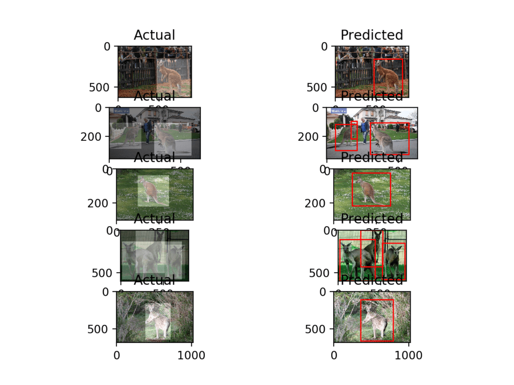
Running the example first creates a figure showing five photos from the training dataset with the ground truth bounding boxes, with the same photo and the predicted bounding boxes alongside.
We can see that the model has done well on these examples, finding all of the kangaroos, even in the case where there are two or three in one photo. The second photo down (in the right column) does show a slip-up where the model has predicted a bounding box around the same kangaroo twice.
Plot of Photos of Kangaroos From the Training Dataset With Ground Truth and Predicted Bounding Boxes
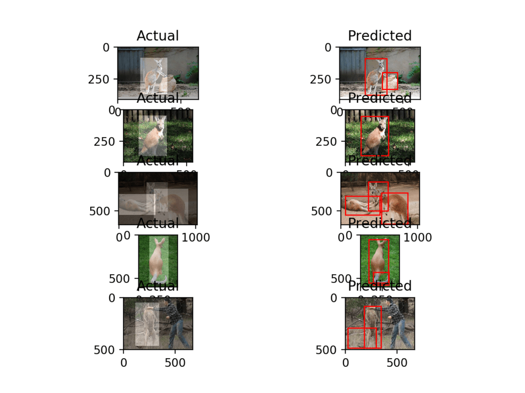
A second figure is created showing five photos from the test dataset with ground truth bounding boxes and predicted bounding boxes.
These are images not seen during training, and again, in each photo, the model has detected the kangaroo. We can see that in the case of the second last photo that a minor mistake was made. Specifically, the same kangaroo was detected multiple times.
No doubt these differences can be ironed out with more training, perhaps with a larger dataset and/or data augmentation, to encourage the model to detect people as background and to detect a given kangaroo once only.
Plot of Photos of Kangaroos From the Training Dataset With Ground Truth and Predicted Bounding Boxes
Further Reading
This section provides more resources on the topic if you are looking to go deeper.