
Author: Jason Brownlee
Face recognition is a computer vision task of identifying and verifying a person based on a photograph of their face.
FaceNet is a face recognition system developed in 2015 by researchers at Google that achieved then state-of-the-art results on a range of face recognition benchmark datasets. The FaceNet system can be used broadly thanks to multiple third-party open source implementations of the model and the availability of pre-trained models.
The FaceNet system can be used to extract high-quality features from faces, called face embeddings, that can then be used to train a face identification system.
In this tutorial, you will discover how to develop a face detection system using FaceNet and an SVM classifier to identify people from photographs.
After completing this tutorial, you will know:
- About the FaceNet face recognition system developed by Google and open source implementations and pre-trained models.
- How to prepare a face detection dataset including first extracting faces via a face detection system and then extracting face features via face embeddings.
- How to fit, evaluate, and demonstrate an SVM model to predict identities from faces embeddings.
Let’s get started.

How to Develop a Face Recognition System Using FaceNet in Keras and an SVM Classifier
Photo by Peter Valverde, some rights reserved.
Tutorial Overview
This tutorial is divided into five parts; they are:
- Face Recognition
- FaceNet Model
- How to Load a FaceNet Model in Keras
- How to Detect Faces for Face Recognition
- How to Develop a Face Classification System
Face Recognition
Face recognition is the general task of identifying and verifying people from photographs of their face.
The 2011 book on face recognition titled “Handbook of Face Recognition” describes two main modes for face recognition, as:
- Face Verification. A one-to-one mapping of a given face against a known identity (e.g. is this the person?).
- Face Identification. A one-to-many mapping for a given face against a database of known faces (e.g. who is this person?).
A face recognition system is expected to identify faces present in images and videos automatically. It can operate in either or both of two modes: (1) face verification (or authentication), and (2) face identification (or recognition).
— Page 1, Handbook of Face Recognition. 2011.
We will focus on the face identification task in this tutorial.
Want Results with Deep Learning for Computer Vision?
Take my free 7-day email crash course now (with sample code).
Click to sign-up and also get a free PDF Ebook version of the course.
FaceNet Model
FaceNet is a face recognition system that was described by Florian Schroff, et al. at Google in their 2015 paper titled “FaceNet: A Unified Embedding for Face Recognition and Clustering.”
It is a system that, given a picture of a face, will extract high-quality features from the face and predict a 128 element vector representation these features, called a face embedding.
FaceNet, that directly learns a mapping from face images to a compact Euclidean space where distances directly correspond to a measure of face similarity.
— FaceNet: A Unified Embedding for Face Recognition and Clustering, 2015.
The model is a deep convolutional neural network trained via a triplet loss function that encourages vectors for the same identity to become more similar (smaller distance), whereas vectors for different identities are expected to become less similar (larger distance). The focus on training a model to create embeddings directly (rather than extracting them from an intermediate layer of a model) was an important innovation in this work.
Our method uses a deep convolutional network trained to directly optimize the embedding itself, rather than an intermediate bottleneck layer as in previous deep learning approaches.
— FaceNet: A Unified Embedding for Face Recognition and Clustering, 2015.
These face embeddings were then used as the basis for training classifier systems on standard face recognition benchmark datasets, achieving then-state-of-the-art results.
Our system cuts the error rate in comparison to the best published result by 30% …
— FaceNet: A Unified Embedding for Face Recognition and Clustering, 2015.
The paper also explores other uses of the embeddings, such as clustering to group like-faces based on their extracted features.
It is a robust and effective face recognition system, and the general nature of the extracted face embeddings lends the approach to a range of applications.
How to Load a FaceNet Model in Keras
There are a number of projects that provide tools to train FaceNet-based models and make use of pre-trained models.
Perhaps the most prominent is called OpenFace that provides FaceNet models built and trained using the PyTorch deep learning framework. There is a port of OpenFace to Keras, called Keras OpenFace, but at the time of writing, the models appear to require Python 2, which is quite limiting.
Another prominent project is called FaceNet by David Sandberg that provides FaceNet models built and trained using TensorFlow. The project looks mature, although at the time of writing does not provide a library-based installation nor clean API. Usefully, David’s project provides a number of high-performing pre-trained FaceNet models and there are a number of projects that port or convert these models for use in Keras.
A notable example is Keras FaceNet by Hiroki Taniai. His project provides a script for converting the Inception ResNet v1 model from TensorFlow to Keras. He also provides a pre-trained Keras model ready for use.
We will use the pre-trained Keras FaceNet model provided by Hiroki Taniai in this tutorial. It was trained on MS-Celeb-1M dataset and expects input images to be color, to have their pixel values whitened (standardized across all three channels), and to have a square shape of 160×160 pixels.
The model can be downloaded from here:
Download the model file and place it in your current working directory with the filename ‘facenet_keras.h5‘.
We can load the model directly in Keras using the load_model() function; for example:
# example of loading the keras facenet model
from keras.models import load_model
# load the model
model = load_model('facenet_keras.h5')
# summarize input and output shape
print(model.inputs)
print(model.outputs)
Running the example loads the model and prints the shape of the input and output tensors.
We can see that the model indeed expects square color images as input with the shape 160×160, and will output a face embedding as a 128 element vector.
# [] # [ ]
Now that we have a FaceNet model, we can explore using it.
How to Detect Faces for Face Recognition
Before we can perform face recognition, we need to detect faces.
Face detection is the process of automatically locating faces in a photograph and localizing them by drawing a bounding box around their extent.
In this tutorial, we will also use the Multi-Task Cascaded Convolutional Neural Network, or MTCNN, for face detection, e.g. finding and extracting faces from photos. This is a state-of-the-art deep learning model for face detection, described in the 2016 paper titled “Joint Face Detection and Alignment Using Multitask Cascaded Convolutional Networks.”
We will use the implementation provided by Iván de Paz Centeno in the ipazc/mtcnn project. This can also be installed via pip as follows:
sudo pip install mtcnn
We can confirm that the library was installed correctly by importing the library and printing the version; for example:
# confirm mtcnn was installed correctly
import mtcnn
# print version
print(mtcnn.__version__)
Running the example prints the current version of the library.
0.0.8
We can use the mtcnn library to create a face detector and extract faces for our use with the FaceNet face detector models in subsequent sections.
The first step is to load an image as a NumPy array, which we can achieve using the PIL library and the open() function. We will also convert the image to RGB, just in case the image has an alpha channel or is black and white.
# load image from file
image = Image.open(filename)
# convert to RGB, if needed
image = image.convert('RGB')
# convert to array
pixels = asarray(image)
Next, we can create an MTCNN face detector class and use it to detect all faces in the loaded photograph.
# create the detector, using default weights
detector = MTCNN()
# detect faces in the image
results = detector.detect_faces(pixels)
The result is a list of bounding boxes, where each bounding box defines a lower-left-corner of the bounding box, as well as the width and height.
If we assume there is only one face in the photo for our experiments, we can determine the pixel coordinates of the bounding box as follows. Sometimes the library will return a negative pixel index, and I think this is a bug. We can fix this by taking the absolute value of the coordinates.
# extract the bounding box from the first face
x1, y1, width, height = results[0]['box']
# bug fix
x1, y1 = abs(x1), abs(y1)
x2, y2 = x1 + width, y1 + height
We can use these coordinates to extract the face.
# extract the face
face = pixels[y1:y2, x1:x2]
We can then use the PIL library to resize this small image of the face to the required size; specifically, the model expects square input faces with the shape 160×160.
# resize pixels to the model size
image = Image.fromarray(face)
image = image.resize((160, 160))
face_array = asarray(image)
Tying all of this together, the function extract_face() will load a photograph from the loaded filename and return the extracted face. It assumes that the photo contains one face and will return the first face detected.
# function for face detection with mtcnn
from PIL import Image
from numpy import asarray
from mtcnn.mtcnn import MTCNN

# extract a single face from a given photograph
def extract_face(filename, required_size=(160, 160)):
	# load image from file
	image = Image.open(filename)
	# convert to RGB, if needed
	image = image.convert('RGB')
	# convert to array
	pixels = asarray(image)
	# create the detector, using default weights
	detector = MTCNN()
	# detect faces in the image
	results = detector.detect_faces(pixels)
	# extract the bounding box from the first face
	x1, y1, width, height = results[0]['box']
	# bug fix
	x1, y1 = abs(x1), abs(y1)
	x2, y2 = x1 + width, y1 + height
	# extract the face
	face = pixels[y1:y2, x1:x2]
	# resize pixels to the model size
	image = Image.fromarray(face)
	image = image.resize(required_size)
	face_array = asarray(image)
	return face_array

# load the photo and extract the face
pixels = extract_face('...')
We can use this function to extract faces as needed in the next section that can be provided as input to the FaceNet model.
How to Develop a Face Classification System
In this section, we will develop a face detection system to predict the identity of a given face.
The model will be trained and tested using the ‘5 Celebrity Faces Dataset‘ that contains many photographs of five different celebrities.
We will use an MTCNN model for face detection, the FaceNet model will be used to create a face embedding for each detected face, then we will develop a Linear Support Vector Machine (SVM) classifier model to predict the identity of a given face.
5 Celebrity Faces Dataset
The 5 Celebrity Faces Dataset is a small dataset that contains photographs of celebrities.
It includes photos of: Ben Affleck, Elton John, Jerry Seinfeld, Madonna, and Mindy Kaling.
The dataset was prepared and made available by Dan Becker and provided for free download on Kaggle. Note, a Kaggle account is required to download the dataset.
Download the dataset (this may require a Kaggle login), data.zip (2.5 megabytes), and unzip it in your local directory with the folder name ‘5-celebrity-faces-dataset‘.
You should now have a directory with the following structure (note, there are spelling mistakes in some directory names, and they were left as-is in this example):
5-celebrity-faces-dataset
├── train
│   ├── ben_afflek
│   ├── elton_john
│   ├── jerry_seinfeld
│   ├── madonna
│   └── mindy_kaling
└── val
    ├── ben_afflek
    ├── elton_john
    ├── jerry_seinfeld
    ├── madonna
    └── mindy_kaling
We can see that there is a training dataset and a validation or test dataset.
Looking at some of the photos in the directories, we can see that the photos provide faces with a range of orientations, lighting, and in various sizes. Importantly, each photo contains one face of the person.
We will use this dataset as the basis for our classifier, trained on the ‘train‘ dataset only and classify faces in the ‘val‘ dataset. You can use this same structure to develop a classifier with your own photographs.
Detect Faces
The first step is to detect the face in each photograph and reduce the dataset to a series of faces only.
Let’s test out our face detector function defined in the previous section, specifically extract_face().
Looking in the ‘5-celebrity-faces-dataset/train/ben_afflek/‘ directory, we can see that there are 14 photographs of Ben Affleck in the training dataset. We can detect the face in each photograph, and create a plot with 14 faces, with two rows of seven images each.
The complete example is listed below.
# demonstrate face detection on 5 Celebrity Faces Dataset
from os import listdir
from PIL import Image
from numpy import asarray
from matplotlib import pyplot
from mtcnn.mtcnn import MTCNN

# extract a single face from a given photograph
def extract_face(filename, required_size=(160, 160)):
	# load image from file
	image = Image.open(filename)
	# convert to RGB, if needed
	image = image.convert('RGB')
	# convert to array
	pixels = asarray(image)
	# create the detector, using default weights
	detector = MTCNN()
	# detect faces in the image
	results = detector.detect_faces(pixels)
	# extract the bounding box from the first face
	x1, y1, width, height = results[0]['box']
	# bug fix
	x1, y1 = abs(x1), abs(y1)
	x2, y2 = x1 + width, y1 + height
	# extract the face
	face = pixels[y1:y2, x1:x2]
	# resize pixels to the model size
	image = Image.fromarray(face)
	image = image.resize(required_size)
	face_array = asarray(image)
	return face_array

# specify folder to plot
folder = '5-celebrity-faces-dataset/train/ben_afflek/'
i = 1
# enumerate files
for filename in listdir(folder):
	# path
	path = folder + filename
	# get face
	face = extract_face(path)
	print(i, face.shape)
	# plot
	pyplot.subplot(2, 7, i)
	pyplot.axis('off')
	pyplot.imshow(face)
	i += 1
pyplot.show()
Running the example takes a moment and reports the progress of each loaded photograph along the way and the shape of the NumPy array containing the face pixel data.
1 (160, 160, 3)
2 (160, 160, 3)
3 (160, 160, 3)
4 (160, 160, 3)
5 (160, 160, 3)
6 (160, 160, 3)
7 (160, 160, 3)
8 (160, 160, 3)
9 (160, 160, 3)
10 (160, 160, 3)
11 (160, 160, 3)
12 (160, 160, 3)
13 (160, 160, 3)
14 (160, 160, 3)
A figure is created containing the faces detected in the Ben Affleck directory.
We can see that each face was correctly detected and that we have a range of lighting, skin tones, and orientations in the detected faces.
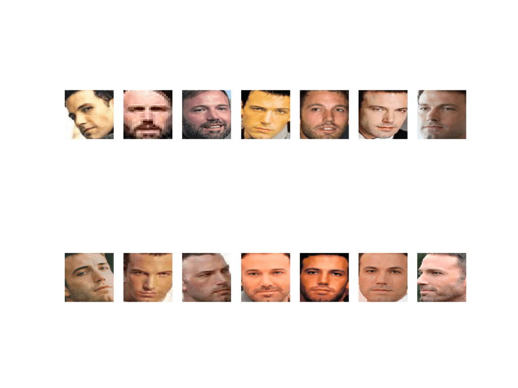
Plot of 14 Faces of Ben Affleck Detected From the Training Dataset of the 5 Celebrity Faces Dataset
So far, so good.
Next, we can extend this example to step over each subdirectory for a given dataset (e.g. ‘train‘ or ‘val‘), extract the faces, and prepare a dataset with the name as the output label for each detected face.
The load_faces() function below will load all of the faces into a list for a given directory, e.g. ‘5-celebrity-faces-dataset/train/ben_afflek/‘.
# load images and extract faces for all images in a directory
def load_faces(directory):
	faces = list()
	# enumerate files
	for filename in listdir(directory):
		# path
		path = directory + filename
		# get face
		face = extract_face(path)
		# store
		faces.append(face)
	return faces
We can call the load_faces() function for each subdirectory in the ‘train‘ or ‘val‘ folders. Each face has one label, the name of the celebrity, which we can take from the directory name.
The load_dataset() function below takes a directory name such as ‘5-celebrity-faces-dataset/train/‘ and detects faces for each subdirectory (celebrity), assigning labels to each detected face.
It returns the X and y elements of the dataset as NumPy arrays.
# load a dataset that contains one subdir for each class that in turn contains images
def load_dataset(directory):
	X, y = list(), list()
	# enumerate folders, on per class
	for subdir in listdir(directory):
		# path
		path = directory + subdir + '/'
		# skip any files that might be in the dir
		if not isdir(path):
			continue
		# load all faces in the subdirectory
		faces = load_faces(path)
		# create labels
		labels = [subdir for _ in range(len(faces))]
		# summarize progress
		print('>loaded %d examples for class: %s' % (len(faces), subdir))
		# store
		X.extend(faces)
		y.extend(labels)
	return asarray(X), asarray(y)
We can then call this function for the ‘train’ and ‘val’ folders to load all of the data, then save the results in a single compressed NumPy array file via the savez_compressed() function.
# load train dataset
trainX, trainy = load_dataset('5-celebrity-faces-dataset/train/')
print(trainX.shape, trainy.shape)
# load test dataset
testX, testy = load_dataset('5-celebrity-faces-dataset/val/')
print(testX.shape, testy.shape)
# save arrays to one file in compressed format
savez_compressed('5-celebrity-faces-dataset.npz', trainX, trainy, testX, testy)
Tying all of this together, the complete example of detecting all of the faces in the 5 Celebrity Faces Dataset is listed below.
# face detection for the 5 Celebrity Faces Dataset
from os import listdir
from os.path import isdir
from PIL import Image
from matplotlib import pyplot
from numpy import savez_compressed
from numpy import asarray
from mtcnn.mtcnn import MTCNN

# extract a single face from a given photograph
def extract_face(filename, required_size=(160, 160)):
	# load image from file
	image = Image.open(filename)
	# convert to RGB, if needed
	image = image.convert('RGB')
	# convert to array
	pixels = asarray(image)
	# create the detector, using default weights
	detector = MTCNN()
	# detect faces in the image
	results = detector.detect_faces(pixels)
	# extract the bounding box from the first face
	x1, y1, width, height = results[0]['box']
	# bug fix
	x1, y1 = abs(x1), abs(y1)
	x2, y2 = x1 + width, y1 + height
	# extract the face
	face = pixels[y1:y2, x1:x2]
	# resize pixels to the model size
	image = Image.fromarray(face)
	image = image.resize(required_size)
	face_array = asarray(image)
	return face_array

# load images and extract faces for all images in a directory
def load_faces(directory):
	faces = list()
	# enumerate files
	for filename in listdir(directory):
		# path
		path = directory + filename
		# get face
		face = extract_face(path)
		# store
		faces.append(face)
	return faces

# load a dataset that contains one subdir for each class that in turn contains images
def load_dataset(directory):
	X, y = list(), list()
	# enumerate folders, on per class
	for subdir in listdir(directory):
		# path
		path = directory + subdir + '/'
		# skip any files that might be in the dir
		if not isdir(path):
			continue
		# load all faces in the subdirectory
		faces = load_faces(path)
		# create labels
		labels = [subdir for _ in range(len(faces))]
		# summarize progress
		print('>loaded %d examples for class: %s' % (len(faces), subdir))
		# store
		X.extend(faces)
		y.extend(labels)
	return asarray(X), asarray(y)

# load train dataset
trainX, trainy = load_dataset('5-celebrity-faces-dataset/train/')
print(trainX.shape, trainy.shape)
# load test dataset
testX, testy = load_dataset('5-celebrity-faces-dataset/val/')
# save arrays to one file in compressed format
savez_compressed('5-celebrity-faces-dataset.npz', trainX, trainy, testX, testy)
Running the example may take a moment.
First, all of the photos in the ‘train‘ dataset are loaded, then faces are extracted, resulting in 93 samples with square face input and a class label string as output. Then the ‘val‘ dataset is loaded, providing 25 samples that can be used as a test dataset.
Both datasets are then saved to a compressed NumPy array file called ‘5-celebrity-faces-dataset.npz‘ that is about three megabytes and is stored in the current working directory.
>loaded 14 examples for class: ben_afflek
>loaded 19 examples for class: madonna
>loaded 17 examples for class: elton_john
>loaded 22 examples for class: mindy_kaling
>loaded 21 examples for class: jerry_seinfeld
(93, 160, 160, 3) (93,)
>loaded 5 examples for class: ben_afflek
>loaded 5 examples for class: madonna
>loaded 5 examples for class: elton_john
>loaded 5 examples for class: mindy_kaling
>loaded 5 examples for class: jerry_seinfeld
(25, 160, 160, 3) (25,)
This dataset is ready to be provided to a face detection model.
Create Face Embeddings
The next step is to create a face embedding.
A face embedding is a vector that represents the features extracted from the face. This can then be compared with the vectors generated for other faces. For example, another vector that is close (by some measure) may be the same person, whereas another vector that is far (by some measure) may be a different person.
The classifier model that we want to develop will take a face embedding as input and predict the identity of the face. The FaceNet model will generate this embedding for a given image of a face.
The FaceNet model can be used as part of the classifier itself, or we can use the FaceNet model to pre-process a face to create a face embedding that can be stored and used as input to our classifier model. This latter approach is preferred as the FaceNet model is both large and slow to create a face embedding.
We can, therefore, pre-compute the face embeddings for all faces in the train and test (formally ‘val‘) sets in our 5 Celebrity Faces Dataset.
First, we can load our detected faces dataset using the load() NumPy function.
# load the face dataset
data = load('5-celebrity-faces-dataset.npz')
trainX, trainy, testX, testy = data['arr_0'], data['arr_1'], data['arr_2'], data['arr_3']
print('Loaded: ', trainX.shape, trainy.shape, testX.shape, testy.shape)
Next, we can load our FaceNet model ready for converting faces into face embeddings.
# load the facenet model
model = load_model('facenet_keras.h5')
print('Loaded Model')
We can then enumerate each face in the train and test datasets to predict an embedding.
To predict an embedding, first the pixel values of the image need to be suitably prepared to meet the expectations of the FaceNet model. This specific implementation of the FaceNet model expects that the pixel values are standardized.
# scale pixel values
face_pixels = face_pixels.astype('float32')
# standardize pixel values across channels (global)
mean, std = face_pixels.mean(), face_pixels.std()
face_pixels = (face_pixels - mean) / std
In order to make a prediction for one example in Keras, we must expand the dimensions so that the face array is one sample.
# transform face into one sample
samples = expand_dims(face_pixels, axis=0)
We can then use the model to make a prediction and extract the embedding vector.
# make prediction to get embedding
yhat = model.predict(samples)
# get embedding
embedding = yhat[0]
The get_embedding() function defined below implements these behaviors and will return a face embedding given a single image of a face and the loaded FaceNet model.
# get the face embedding for one face
def get_embedding(model, face_pixels):
	# scale pixel values
	face_pixels = face_pixels.astype('float32')
	# standardize pixel values across channels (global)
	mean, std = face_pixels.mean(), face_pixels.std()
	face_pixels = (face_pixels - mean) / std
	# transform face into one sample
	samples = expand_dims(face_pixels, axis=0)
	# make prediction to get embedding
	yhat = model.predict(samples)
	return yhat[0]
Tying all of this together, the complete example of converting each face into a face embedding in the train and test datasets is listed below.
# calculate a face embedding for each face in the dataset using facenet
from numpy import load
from numpy import expand_dims
from numpy import asarray
from numpy import savez_compressed
from keras.models import load_model

# get the face embedding for one face
def get_embedding(model, face_pixels):
	# scale pixel values
	face_pixels = face_pixels.astype('float32')
	# standardize pixel values across channels (global)
	mean, std = face_pixels.mean(), face_pixels.std()
	face_pixels = (face_pixels - mean) / std
	# transform face into one sample
	samples = expand_dims(face_pixels, axis=0)
	# make prediction to get embedding
	yhat = model.predict(samples)
	return yhat[0]

# load the face dataset
data = load('5-celebrity-faces-dataset.npz')
trainX, trainy, testX, testy = data['arr_0'], data['arr_1'], data['arr_2'], data['arr_3']
print('Loaded: ', trainX.shape, trainy.shape, testX.shape, testy.shape)
# load the facenet model
model = load_model('facenet_keras.h5')
print('Loaded Model')
# convert each face in the train set to an embedding
newTrainX = list()
for face_pixels in trainX:
	embedding = get_embedding(model, face_pixels)
	newTrainX.append(embedding)
newTrainX = asarray(newTrainX)
print(newTrainX.shape)
# convert each face in the test set to an embedding
newTestX = list()
for face_pixels in testX:
	embedding = get_embedding(model, face_pixels)
	newTestX.append(embedding)
newTestX = asarray(newTestX)
print(newTestX.shape)
# save arrays to one file in compressed format
savez_compressed('5-celebrity-faces-embeddings.npz', newTrainX, trainy, newTestX, testy)
Running the example reports progress along the way.
We can see that the face dataset was loaded correctly and so was the model. The train dataset was then transformed into 93 face embeddings, each comprised of a 128 element vector. The 25 examples in the test dataset were also suitably converted to face embeddings.
The resulting datasets were then saved to a compressed NumPy array that is about 50 kilobytes with the name ‘5-celebrity-faces-embeddings.npz‘ in the current working directory.
Loaded:  (93, 160, 160, 3) (93,) (25, 160, 160, 3) (25,)
Loaded Model
(93, 128)
(25, 128)
We are now ready to develop our face classifier system.
Perform Face Classification
In this section, we will develop a model to classify face embeddings as one of the known celebrities in the 5 Celebrity Faces Dataset.
First, we must load the face embeddings dataset.
# load dataset
data = load('5-celebrity-faces-embeddings.npz')
trainX, trainy, testX, testy = data['arr_0'], data['arr_1'], data['arr_2'], data['arr_3']
print('Dataset: train=%d, test=%d' % (trainX.shape[0], testX.shape[0]))
Next, the data requires some minor preparation prior to modeling.
First, it is a good practice to normalize the face embedding vectors. It is a good practice because the vectors are often compared to each other using a distance metric.
In this context, vector normalization means scaling the values until the length or magnitude of the vectors is 1 or unit length. This can be achieved using the Normalizer class in scikit-learn. It might even be more convenient to perform this step when the face embeddings are created in the previous step.
# normalize input vectors
in_encoder = Normalizer(norm='l2')
trainX = in_encoder.transform(trainX)
testX = in_encoder.transform(testX)
Next, the string target variables for each celebrity name need to be converted to integers.
This can be achieved via the LabelEncoder class in scikit-learn.
# label encode targets
out_encoder = LabelEncoder()
out_encoder.fit(trainy)
trainy = out_encoder.transform(trainy)
testy = out_encoder.transform(testy)
Next, we can fit a model.
It is common to use a Linear Support Vector Machine (SVM) when working with normalized face embedding inputs. This is because the method is very effective at separating the face embedding vectors. We can fit a linear SVM to the training data using the SVC class in scikit-learn and setting the ‘kernel‘ attribute to ‘linear‘. We may also want probabilities later when making predictions, which can be configured by setting ‘probability‘ to ‘True‘.
# fit model
model = SVC(kernel='linear')
model.fit(trainX, trainy)
Next, we can evaluate the model.
This can be achieved by using the fit model to make a prediction for each example in the train and test datasets and then calculating the classification accuracy.
# predict
yhat_train = model.predict(trainX)
yhat_test = model.predict(testX)
# score
score_train = accuracy_score(trainy, yhat_train)
score_test = accuracy_score(testy, yhat_test)
# summarize
print('Accuracy: train=%.3f, test=%.3f' % (score_train*100, score_test*100))
Tying all of this together, the complete example of fitting a Linear SVM on the face embeddings for the 5 Celebrity Faces Dataset is listed below.
# develop a classifier for the 5 Celebrity Faces Dataset
from numpy import load
from sklearn.metrics import accuracy_score
from sklearn.preprocessing import LabelEncoder
from sklearn.preprocessing import Normalizer
from sklearn.svm import SVC
# load dataset
data = load('5-celebrity-faces-embeddings.npz')
trainX, trainy, testX, testy = data['arr_0'], data['arr_1'], data['arr_2'], data['arr_3']
print('Dataset: train=%d, test=%d' % (trainX.shape[0], testX.shape[0]))
# normalize input vectors
in_encoder = Normalizer(norm='l2')
trainX = in_encoder.transform(trainX)
testX = in_encoder.transform(testX)
# label encode targets
out_encoder = LabelEncoder()
out_encoder.fit(trainy)
trainy = out_encoder.transform(trainy)
testy = out_encoder.transform(testy)
# fit model
model = SVC(kernel='linear', probability=True)
model.fit(trainX, trainy)
# predict
yhat_train = model.predict(trainX)
yhat_test = model.predict(testX)
# score
score_train = accuracy_score(trainy, yhat_train)
score_test = accuracy_score(testy, yhat_test)
# summarize
print('Accuracy: train=%.3f, test=%.3f' % (score_train*100, score_test*100))
Running the example first confirms that the number of samples in the train and test datasets is as we expect
Next, the model is evaluated on the train and test dataset, showing perfect classification accuracy. This is not surprising given the size of the dataset and the power of the face detection and face recognition models used.
Dataset: train=93, test=25
Accuracy: train=100.000, test=100.000
We can make it more interesting by plotting the original face and the prediction.
First, we need to load the face dataset, specifically the faces in the test dataset. We could also load the original photos to make it even more interesting.
# load faces
data = load('5-celebrity-faces-dataset.npz')
testX_faces = data['arr_2']
The rest of the example is the same up until we fit the model.
First, we need to select a random example from the test set, then get the embedding, face pixels, expected class prediction, and the corresponding name for the class.
# test model on a random example from the test dataset
selection = choice([i for i in range(testX.shape[0])])
random_face_pixels = testX_faces[selection]
random_face_emb = testX[selection]
random_face_class = testy[selection]
random_face_name = out_encoder.inverse_transform([random_face_class])
Next, we can use the face embedding as an input to make a single prediction with the fit model.
We can predict both the class integer and the probability of the prediction.
# prediction for the face
samples = expand_dims(random_face_emb, axis=0)
yhat_class = model.predict(samples)
yhat_prob = model.predict_proba(samples)
We can then get the name for the predicted class integer, and the probability for this prediction.
# get name
class_index = yhat_class[0]
class_probability = yhat_prob[0,class_index] * 100
predict_names = out_encoder.inverse_transform(yhat_class)
We can then print this information.
print('Predicted: %s (%.3f)' % (predict_names[0], class_probability))
print('Expected: %s' % random_face_name[0])
We can also plot the face pixels along with the predicted name and probability.
# plot for fun
pyplot.imshow(random_face_pixels)
title = '%s (%.3f)' % (predict_names[0], class_probability)
pyplot.title(title)
pyplot.show()
Tying all of this together, the complete example for predicting the identity for a given unseen photo in the test dataset is listed below.
# develop a classifier for the 5 Celebrity Faces Dataset
from random import choice
from numpy import load
from numpy import expand_dims
from sklearn.preprocessing import LabelEncoder
from sklearn.preprocessing import Normalizer
from sklearn.svm import SVC
from matplotlib import pyplot
# load faces
data = load('5-celebrity-faces-dataset.npz')
testX_faces = data['arr_2']
# load face embeddings
data = load('5-celebrity-faces-embeddings.npz')
trainX, trainy, testX, testy = data['arr_0'], data['arr_1'], data['arr_2'], data['arr_3']
# normalize input vectors
in_encoder = Normalizer(norm='l2')
trainX = in_encoder.transform(trainX)
testX = in_encoder.transform(testX)
# label encode targets
out_encoder = LabelEncoder()
out_encoder.fit(trainy)
trainy = out_encoder.transform(trainy)
testy = out_encoder.transform(testy)
# fit model
model = SVC(kernel='linear', probability=True)
model.fit(trainX, trainy)
# test model on a random example from the test dataset
selection = choice([i for i in range(testX.shape[0])])
random_face_pixels = testX_faces[selection]
random_face_emb = testX[selection]
random_face_class = testy[selection]
random_face_name = out_encoder.inverse_transform([random_face_class])
# prediction for the face
samples = expand_dims(random_face_emb, axis=0)
yhat_class = model.predict(samples)
yhat_prob = model.predict_proba(samples)
# get name
class_index = yhat_class[0]
class_probability = yhat_prob[0,class_index] * 100
predict_names = out_encoder.inverse_transform(yhat_class)
print('Predicted: %s (%.3f)' % (predict_names[0], class_probability))
print('Expected: %s' % random_face_name[0])
# plot for fun
pyplot.imshow(random_face_pixels)
title = '%s (%.3f)' % (predict_names[0], class_probability)
pyplot.title(title)
pyplot.show()
A different random example from the test dataset will be selected each time the code is run.
Try running it a few times.
In this case, a photo of Jerry Seinfeld is selected and correctly predicted.
Predicted: jerry_seinfeld (88.476)
Expected: jerry_seinfeld
A plot of the chosen face is also created, showing the predicted name and probability in the image title.
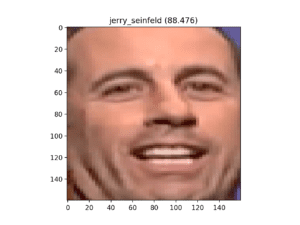
Detected Face of Jerry Seinfeld, Correctly Identified by the SVM Classifier
Further Reading
This section provides more resources on the topic if you are looking to go deeper.
Papers
Books
Projects
- OpenFace PyTorch Project.
- OpenFace Keras Project, GitHub.
- Keras FaceNet Project, GitHub.
- MS-Celeb 1M Dataset.
APIs
Summary
In this tutorial, you discovered how to develop a face detection system using FaceNet and an SVM classifier to identify people from photographs.
Specifically, you learned:
- About the FaceNet face recognition system developed by Google and open source implementations and pre-trained models.
- How to prepare a face detection dataset including first extracting faces via a face detection system and then extracting face features via face embeddings.
- How to fit, evaluate, and demonstrate an SVM model to predict identities from faces embeddings.
Do you have any questions?
Ask your questions in the comments below and I will do my best to answer.
The post How to Develop a Face Recognition System Using FaceNet in Keras appeared first on Machine Learning Mastery.