Author: Jason Brownlee
How to Identify Unstable Models When Training Generative Adversarial Networks.
GANs are difficult to train.
The reason they are difficult to train is that both the generator model and the discriminator model are trained simultaneously in a zero sum game. This means that improvements to one model come at the expense of the other model.
The goal of training two models involves finding a point of equilibrium between the two competing concerns.
It also means that every time the parameters of one of the models are updated, the nature of the optimization problem that is being solved is changed. This has the effect of creating a dynamic system. In neural network terms, the technical challenge of training two competing neural networks at the same time is that they can fail to converge.
It is important to develop an intuition for both the normal convergence of a GAN model and unusual convergence of GAN models, sometimes called failure modes.
In this tutorial, we will first develop a stable GAN model for a simple image generation task in order to establish what normal convergence looks like and what to expect more generally.
We will then impair the GAN models in different ways and explore a range of failure modes that you may encounter when training GAN models. These scenarios will help you to develop an intuition for what to look for or expect when a GAN model is failing to train, and ideas for what you could do about it.
After completing this tutorial, you will know:
- How to identify a stable GAN training process from the generator and discriminator loss over time.
- How to identify a mode collapse by reviewing both learning curves and generated images.
- How to identify a convergence failure by reviewing learning curves of generator and discriminator loss over time.
Let’s get started.
A Practical Guide to Generative Adversarial Network Failure Modes
Photo by Jason Heavner, some rights reserved.
Tutorial Overview
This tutorial is divided into three parts; they are:
- How To Identify a Stable Generative Adversarial Network
- How To Identify a Mode Collapse in a Generative Adversarial Network
- How To Identify Convergence Failure in a Generative Adversarial Network
How To Train a Stable Generative Adversarial Network
In this section, we will train a stable GAN to generate images of a handwritten digit.
Specifically, we will use the digit ‘8’ from the MNIST handwritten digit dataset.
The results of this model will establish both a stable GAN that can be used for later experimentation and a profile for what generated images and learning curves look like for a stable GAN training process.
The first step is to define the models.
The discriminator model takes as input one 28×28 grayscale image and outputs a binary prediction as to whether the image is real (class=1) or fake (class=0). It is implemented as a modest convolutional neural network using best practices for GAN design such as using the LeakyReLU activation function with a slope of 0.2, batch normalization, using a 2×2 stride to downsample, and the adam version of stochastic gradient descent with a learning rate of 0.0002 and a momentum of 0.5
The define_discriminator() function below implements this, defining and compiling the discriminator model and returning it. The input shape of the image is parameterized as a default function argument to make it clear.
# define the standalone discriminator model
def define_discriminator(in_shape=(28,28,1)):
	# weight initialization
	init = RandomNormal(stddev=0.02)
	# define model
	model = Sequential()
	# downsample to 14x14
	model.add(Conv2D(64, (4,4), strides=(2,2), padding='same', kernel_initializer=init, input_shape=in_shape))
	model.add(BatchNormalization())
	model.add(LeakyReLU(alpha=0.2))
	# downsample to 7x7
	model.add(Conv2D(64, (4,4), strides=(2,2), padding='same', kernel_initializer=init))
	model.add(BatchNormalization())
	model.add(LeakyReLU(alpha=0.2))
	# classifier
	model.add(Flatten())
	model.add(Dense(1, activation='sigmoid'))
	# compile model
	opt = Adam(lr=0.0002, beta_1=0.5)
	model.compile(loss='binary_crossentropy', optimizer=opt, metrics=['accuracy'])
	return model
The generator model takes as input a point in the latent space and outputs a single 28×28 grayscale image. This is achieved by using a fully connected layer to interpret the point in the latent space and provide sufficient activations that can be reshaped into many copies (in this case, 128) of a low-resolution version of the output image (e.g. 7×7). This is then upsampled two times, doubling the size and quadrupling the area of the activations each time using transpose convolutional layers. The model uses best practices such as the LeakyReLU activation, a kernel size that is a factor of the stride size, and a hyperbolic tangent (tanh) activation function in the output layer.
The define_generator() function below defines the generator model, but intentionally does not compile it as it is not trained directly, then returns the model. The size of the latent space is parameterized as a function argument.
# define the standalone generator model
def define_generator(latent_dim):
	# weight initialization
	init = RandomNormal(stddev=0.02)
	# define model
	model = Sequential()
	# foundation for 7x7 image
	n_nodes = 128 * 7 * 7
	model.add(Dense(n_nodes, kernel_initializer=init, input_dim=latent_dim))
	model.add(LeakyReLU(alpha=0.2))
	model.add(Reshape((7, 7, 128)))
	# upsample to 14x14
	model.add(Conv2DTranspose(128, (4,4), strides=(2,2), padding='same', kernel_initializer=init))
	model.add(BatchNormalization())
	model.add(LeakyReLU(alpha=0.2))
	# upsample to 28x28
	model.add(Conv2DTranspose(128, (4,4), strides=(2,2), padding='same', kernel_initializer=init))
	model.add(BatchNormalization())
	model.add(LeakyReLU(alpha=0.2))
	# output 28x28x1
	model.add(Conv2D(1, (7,7), activation='tanh', padding='same', kernel_initializer=init))
	return model
Next, a GAN model can be defined that combines both the generator model and the discriminator model into one larger model. This larger model will be used to train the model weights in the generator, using the output and error calculated by the discriminator model. The discriminator model is trained separately, and as such, the model weights are marked as not trainable in this larger GAN model to ensure that only the weights of the generator model are updated. This change to the trainability of the discriminator weights only has an effect when training the combined GAN model, not when training the discriminator standalone.
This larger GAN model takes as input a point in the latent space, uses the generator model to generate an image, which is fed as input to the discriminator model, then output or classified as real or fake.
The define_gan() function below implements this, taking the already defined generator and discriminator models as input.
# define the combined generator and discriminator model, for updating the generator
def define_gan(generator, discriminator):
	# make weights in the discriminator not trainable
	discriminator.trainable = False
	# connect them
	model = Sequential()
	# add generator
	model.add(generator)
	# add the discriminator
	model.add(discriminator)
	# compile model
	opt = Adam(lr=0.0002, beta_1=0.5)
	model.compile(loss='binary_crossentropy', optimizer=opt)
	return model
Now that we have defined the GAN model, we need to train it. But, before we can train the model, we require input data.
The first step is to load and scale the MNIST dataset. The whole dataset is loaded via a call to the load_data() Keras function, then a subset of the images are selected (about 5,000) that belong to class 8, e.g. are a handwritten depiction of the number eight. Then the pixel values must be scaled to the range [-1,1] to match the output of the generator model.
The load_real_samples() function below implements this, returning the loaded and scaled subset of the MNIST training dataset ready for modeling.
# load mnist images
def load_real_samples():
	# load dataset
	(trainX, trainy), (_, _) = load_data()
	# expand to 3d, e.g. add channels
	X = expand_dims(trainX, axis=-1)
	# select all of the examples for a given class
	selected_ix = trainy == 8
	X = X[selected_ix]
	# convert from ints to floats
	X = X.astype('float32')
	# scale from [0,255] to [-1,1]
	X = (X - 127.5) / 127.5
	return X
We will require one (or a half) batch of real images from the dataset each update to the GAN model. A simple way to achieve this is to select a random sample of images from the dataset each time.
The generate_real_samples() function below implements this, taking the prepared dataset as an argument, selecting and returning a random sample of face images, and their corresponding class label for the discriminator, specifically class=1 indicating that they are real images.
# select real samples
def generate_real_samples(dataset, n_samples):
	# choose random instances
	ix = randint(0, dataset.shape[0], n_samples)
	# select images
	X = dataset[ix]
	# generate class labels
	y = ones((n_samples, 1))
	return X, y
Next, we need inputs for the generator model. These are random points from the latent space, specifically Gaussian distributed random variables.
The generate_latent_points() function implements this, taking the size of the latent space as an argument and the number of points required, and returning them as a batch of input samples for the generator model.
# generate points in latent space as input for the generator
def generate_latent_points(latent_dim, n_samples):
	# generate points in the latent space
	x_input = randn(latent_dim * n_samples)
	# reshape into a batch of inputs for the network
	x_input = x_input.reshape(n_samples, latent_dim)
	return x_input
Next, we need to use the points in the latent space as input to the generator in order to generate new images.
The generate_fake_samples() function below implements this, taking the generator model and size of the latent space as arguments, then generating points in the latent space and using them as input to the generator model. The function returns the generated images and their corresponding class label for the discriminator model, specifically class=0 to indicate they are fake or generated.
# use the generator to generate n fake examples, with class labels
def generate_fake_samples(generator, latent_dim, n_samples):
	# generate points in latent space
	x_input = generate_latent_points(latent_dim, n_samples)
	# predict outputs
	X = generator.predict(x_input)
	# create class labels
	y = zeros((n_samples, 1))
	return X, y
We need to record the performance of the model. Perhaps the most reliable way to evaluate the performance of a GAN is to use the generator to generate images, and then review and subjectively evaluate them.
The summarize_performance() function below takes the generator model at a given point during training and uses it to generate 100 images in a 10×10 grid that are then plotted and saved to file. The model is also saved to file at this time, in case we would like to use it later to generate more images.
# generate samples and save as a plot and save the model
def summarize_performance(step, g_model, latent_dim, n_samples=100):
	# prepare fake examples
	X, _ = generate_fake_samples(g_model, latent_dim, n_samples)
	# scale from [-1,1] to [0,1]
	X = (X + 1) / 2.0
	# plot images
	for i in range(10 * 10):
		# define subplot
		pyplot.subplot(10, 10, 1 + i)
		# turn off axis
		pyplot.axis('off')
		# plot raw pixel data
		pyplot.imshow(X[i, :, :, 0], cmap='gray_r')
	# save plot to file
	pyplot.savefig('results_baseline/generated_plot_%03d.png' % (step+1))
	pyplot.close()
	# save the generator model
	g_model.save('results_baseline/model_%03d.h5' % (step+1))
In addition to image quality, it is a good idea to keep track of the loss and accuracy of the model over time.
The loss and classification accuracy for the discriminator for real and fake samples can be tracked for each model update, as can the loss for the generator for each update. These can then be used to create line plots of loss and accuracy at the end of the training run.
The plot_history() function below implements this and saves the results to file.
# create a line plot of loss for the gan and save to file
def plot_history(d1_hist, d2_hist, g_hist, a1_hist, a2_hist):
	# plot loss
	pyplot.subplot(2, 1, 1)
	pyplot.plot(d1_hist, label='d-real')
	pyplot.plot(d2_hist, label='d-fake')
	pyplot.plot(g_hist, label='gen')
	pyplot.legend()
	# plot discriminator accuracy
	pyplot.subplot(2, 1, 2)
	pyplot.plot(a1_hist, label='acc-real')
	pyplot.plot(a2_hist, label='acc-fake')
	pyplot.legend()
	# save plot to file
	pyplot.savefig('results_baseline/plot_line_plot_loss.png')
	pyplot.close()
We are now ready to fit the GAN model.
The model is fit for 10 training epochs, which is arbitrary, as the model begins generating plausible number-8 digits after perhaps the first few epochs. A batch size of 128 samples is used, and each training epoch involves 5,851/128 or about 45 batches of real and fake samples and updates to the model. The model is therefore trained for 10 epochs of 45 batches, or 450 iterations.
First, the discriminator model is updated for a half batch of real samples, then a half batch of fake samples, together forming one batch of weight updates. The generator is then updated via the composite GAN model. Importantly, the class label is set to 1, or real, for the fake samples. This has the effect of updating the generator toward getting better at generating real samples on the next batch.
The train() function below implements this, taking the defined models, dataset, and size of the latent dimension as arguments and parameterizing the number of epochs and batch size with default arguments. The generator model is saved at the end of training.
The performance of the discriminator and generator models is reported each iteration. Sample images are generated and saved every epoch, and line plots of model performance are created and saved at the end of the run.
# train the generator and discriminator
def train(g_model, d_model, gan_model, dataset, latent_dim, n_epochs=10, n_batch=128):
	# calculate the number of batches per epoch
	bat_per_epo = int(dataset.shape[0] / n_batch)
	# calculate the total iterations based on batch and epoch
	n_steps = bat_per_epo * n_epochs
	# calculate the number of samples in half a batch
	half_batch = int(n_batch / 2)
	# prepare lists for storing stats each iteration
	d1_hist, d2_hist, g_hist, a1_hist, a2_hist = list(), list(), list(), list(), list()
	# manually enumerate epochs
	for i in range(n_steps):
		# get randomly selected 'real' samples
		X_real, y_real = generate_real_samples(dataset, half_batch)
		# update discriminator model weights
		d_loss1, d_acc1 = d_model.train_on_batch(X_real, y_real)
		# generate 'fake' examples
		X_fake, y_fake = generate_fake_samples(g_model, latent_dim, half_batch)
		# update discriminator model weights
		d_loss2, d_acc2 = d_model.train_on_batch(X_fake, y_fake)
		# prepare points in latent space as input for the generator
		X_gan = generate_latent_points(latent_dim, n_batch)
		# create inverted labels for the fake samples
		y_gan = ones((n_batch, 1))
		# update the generator via the discriminator's error
		g_loss = gan_model.train_on_batch(X_gan, y_gan)
		# summarize loss on this batch
		print('>%d, d1=%.3f, d2=%.3f g=%.3f, a1=%d, a2=%d' %
			(i+1, d_loss1, d_loss2, g_loss, int(100*d_acc1), int(100*d_acc2)))
		# record history
		d1_hist.append(d_loss1)
		d2_hist.append(d_loss2)
		g_hist.append(g_loss)
		a1_hist.append(d_acc1)
		a2_hist.append(d_acc2)
		# evaluate the model performance every 'epoch'
		if (i+1) % bat_per_epo == 0:
			summarize_performance(i, g_model, latent_dim)
	plot_history(d1_hist, d2_hist, g_hist, a1_hist, a2_hist)
Now that all of the functions have been defined, we can create the directory where images and models will be stored (in this case ‘results_baseline‘), create the models, load the dataset, and begin the training process.
# make folder for results
makedirs('results_baseline', exist_ok=True)
# size of the latent space
latent_dim = 50
# create the discriminator
discriminator = define_discriminator()
# create the generator
generator = define_generator(latent_dim)
# create the gan
gan_model = define_gan(generator, discriminator)
# load image data
dataset = load_real_samples()
print(dataset.shape)
# train model
train(generator, discriminator, gan_model, dataset, latent_dim)
Tying all of this together, the complete example is listed below.
# example of training a stable gan for generating a handwritten digit
from os import makedirs
from numpy import expand_dims
from numpy import zeros
from numpy import ones
from numpy.random import randn
from numpy.random import randint
from keras.datasets.mnist import load_data
from keras.optimizers import Adam
from keras.models import Sequential
from keras.layers import Dense
from keras.layers import Reshape
from keras.layers import Flatten
from keras.layers import Conv2D
from keras.layers import Conv2DTranspose
from keras.layers import LeakyReLU
from keras.layers import BatchNormalization
from keras.initializers import RandomNormal
from matplotlib import pyplot

# define the standalone discriminator model
def define_discriminator(in_shape=(28,28,1)):
	# weight initialization
	init = RandomNormal(stddev=0.02)
	# define model
	model = Sequential()
	# downsample to 14x14
	model.add(Conv2D(64, (4,4), strides=(2,2), padding='same', kernel_initializer=init, input_shape=in_shape))
	model.add(BatchNormalization())
	model.add(LeakyReLU(alpha=0.2))
	# downsample to 7x7
	model.add(Conv2D(64, (4,4), strides=(2,2), padding='same', kernel_initializer=init))
	model.add(BatchNormalization())
	model.add(LeakyReLU(alpha=0.2))
	# classifier
	model.add(Flatten())
	model.add(Dense(1, activation='sigmoid'))
	# compile model
	opt = Adam(lr=0.0002, beta_1=0.5)
	model.compile(loss='binary_crossentropy', optimizer=opt, metrics=['accuracy'])
	return model

# define the standalone generator model
def define_generator(latent_dim):
	# weight initialization
	init = RandomNormal(stddev=0.02)
	# define model
	model = Sequential()
	# foundation for 7x7 image
	n_nodes = 128 * 7 * 7
	model.add(Dense(n_nodes, kernel_initializer=init, input_dim=latent_dim))
	model.add(LeakyReLU(alpha=0.2))
	model.add(Reshape((7, 7, 128)))
	# upsample to 14x14
	model.add(Conv2DTranspose(128, (4,4), strides=(2,2), padding='same', kernel_initializer=init))
	model.add(BatchNormalization())
	model.add(LeakyReLU(alpha=0.2))
	# upsample to 28x28
	model.add(Conv2DTranspose(128, (4,4), strides=(2,2), padding='same', kernel_initializer=init))
	model.add(BatchNormalization())
	model.add(LeakyReLU(alpha=0.2))
	# output 28x28x1
	model.add(Conv2D(1, (7,7), activation='tanh', padding='same', kernel_initializer=init))
	return model

# define the combined generator and discriminator model, for updating the generator
def define_gan(generator, discriminator):
	# make weights in the discriminator not trainable
	discriminator.trainable = False
	# connect them
	model = Sequential()
	# add generator
	model.add(generator)
	# add the discriminator
	model.add(discriminator)
	# compile model
	opt = Adam(lr=0.0002, beta_1=0.5)
	model.compile(loss='binary_crossentropy', optimizer=opt)
	return model

# load mnist images
def load_real_samples():
	# load dataset
	(trainX, trainy), (_, _) = load_data()
	# expand to 3d, e.g. add channels
	X = expand_dims(trainX, axis=-1)
	# select all of the examples for a given class
	selected_ix = trainy == 8
	X = X[selected_ix]
	# convert from ints to floats
	X = X.astype('float32')
	# scale from [0,255] to [-1,1]
	X = (X - 127.5) / 127.5
	return X

# select real samples
def generate_real_samples(dataset, n_samples):
	# choose random instances
	ix = randint(0, dataset.shape[0], n_samples)
	# select images
	X = dataset[ix]
	# generate class labels
	y = ones((n_samples, 1))
	return X, y

# generate points in latent space as input for the generator
def generate_latent_points(latent_dim, n_samples):
	# generate points in the latent space
	x_input = randn(latent_dim * n_samples)
	# reshape into a batch of inputs for the network
	x_input = x_input.reshape(n_samples, latent_dim)
	return x_input

# use the generator to generate n fake examples, with class labels
def generate_fake_samples(generator, latent_dim, n_samples):
	# generate points in latent space
	x_input = generate_latent_points(latent_dim, n_samples)
	# predict outputs
	X = generator.predict(x_input)
	# create class labels
	y = zeros((n_samples, 1))
	return X, y

# generate samples and save as a plot and save the model
def summarize_performance(step, g_model, latent_dim, n_samples=100):
	# prepare fake examples
	X, _ = generate_fake_samples(g_model, latent_dim, n_samples)
	# scale from [-1,1] to [0,1]
	X = (X + 1) / 2.0
	# plot images
	for i in range(10 * 10):
		# define subplot
		pyplot.subplot(10, 10, 1 + i)
		# turn off axis
		pyplot.axis('off')
		# plot raw pixel data
		pyplot.imshow(X[i, :, :, 0], cmap='gray_r')
	# save plot to file
	pyplot.savefig('results_baseline/generated_plot_%03d.png' % (step+1))
	pyplot.close()
	# save the generator model
	g_model.save('results_baseline/model_%03d.h5' % (step+1))

# create a line plot of loss for the gan and save to file
def plot_history(d1_hist, d2_hist, g_hist, a1_hist, a2_hist):
	# plot loss
	pyplot.subplot(2, 1, 1)
	pyplot.plot(d1_hist, label='d-real')
	pyplot.plot(d2_hist, label='d-fake')
	pyplot.plot(g_hist, label='gen')
	pyplot.legend()
	# plot discriminator accuracy
	pyplot.subplot(2, 1, 2)
	pyplot.plot(a1_hist, label='acc-real')
	pyplot.plot(a2_hist, label='acc-fake')
	pyplot.legend()
	# save plot to file
	pyplot.savefig('results_baseline/plot_line_plot_loss.png')
	pyplot.close()

# train the generator and discriminator
def train(g_model, d_model, gan_model, dataset, latent_dim, n_epochs=10, n_batch=128):
	# calculate the number of batches per epoch
	bat_per_epo = int(dataset.shape[0] / n_batch)
	# calculate the total iterations based on batch and epoch
	n_steps = bat_per_epo * n_epochs
	# calculate the number of samples in half a batch
	half_batch = int(n_batch / 2)
	# prepare lists for storing stats each iteration
	d1_hist, d2_hist, g_hist, a1_hist, a2_hist = list(), list(), list(), list(), list()
	# manually enumerate epochs
	for i in range(n_steps):
		# get randomly selected 'real' samples
		X_real, y_real = generate_real_samples(dataset, half_batch)
		# update discriminator model weights
		d_loss1, d_acc1 = d_model.train_on_batch(X_real, y_real)
		# generate 'fake' examples
		X_fake, y_fake = generate_fake_samples(g_model, latent_dim, half_batch)
		# update discriminator model weights
		d_loss2, d_acc2 = d_model.train_on_batch(X_fake, y_fake)
		# prepare points in latent space as input for the generator
		X_gan = generate_latent_points(latent_dim, n_batch)
		# create inverted labels for the fake samples
		y_gan = ones((n_batch, 1))
		# update the generator via the discriminator's error
		g_loss = gan_model.train_on_batch(X_gan, y_gan)
		# summarize loss on this batch
		print('>%d, d1=%.3f, d2=%.3f g=%.3f, a1=%d, a2=%d' %
			(i+1, d_loss1, d_loss2, g_loss, int(100*d_acc1), int(100*d_acc2)))
		# record history
		d1_hist.append(d_loss1)
		d2_hist.append(d_loss2)
		g_hist.append(g_loss)
		a1_hist.append(d_acc1)
		a2_hist.append(d_acc2)
		# evaluate the model performance every 'epoch'
		if (i+1) % bat_per_epo == 0:
			summarize_performance(i, g_model, latent_dim)
	plot_history(d1_hist, d2_hist, g_hist, a1_hist, a2_hist)

# make folder for results
makedirs('results_baseline', exist_ok=True)
# size of the latent space
latent_dim = 50
# create the discriminator
discriminator = define_discriminator()
# create the generator
generator = define_generator(latent_dim)
# create the gan
gan_model = define_gan(generator, discriminator)
# load image data
dataset = load_real_samples()
print(dataset.shape)
# train model
train(generator, discriminator, gan_model, dataset, latent_dim)
Running the example is quick, taking approximately 10 minutes on modern hardware without a GPU.
Your specific results will vary given the stochastic nature of the learning algorithm. Nevertheless, the general structure of training should be very similar.
First, the loss and accuracy of the discriminator and loss for the generator model are reported to the console each iteration of the training loop.
This is important. A stable GAN will have a discriminator loss around 0.5, typically between 0.5 and maybe as high as 0.7 or 0.8. The generator loss is typically higher and may hover around 1.0, 1.5, 2.0, or even higher.
The accuracy of the discriminator on both real and generated (fake) images will not be 50%, but should typically hover around 70% to 80%.
For both the discriminator and generator, behaviors are likely to start off erratic and move around a lot before the model converges to a stable equilibrium.
>1, d1=0.859, d2=0.664 g=0.872, a1=37, a2=59
>2, d1=0.190, d2=1.429 g=0.555, a1=100, a2=10
>3, d1=0.094, d2=1.467 g=0.597, a1=100, a2=4
>4, d1=0.097, d2=1.315 g=0.686, a1=100, a2=9
>5, d1=0.100, d2=1.241 g=0.714, a1=100, a2=9
...
>446, d1=0.593, d2=0.546 g=1.330, a1=76, a2=82
>447, d1=0.551, d2=0.739 g=0.981, a1=82, a2=39
>448, d1=0.628, d2=0.505 g=1.420, a1=79, a2=89
>449, d1=0.641, d2=0.533 g=1.381, a1=60, a2=85
>450, d1=0.550, d2=0.731 g=1.100, a1=76, a2=42
Line plots for loss and accuracy are created and saved at the end of the run.
The figure contains two subplots. The top subplot shows line plots for the discriminator loss for real images (blue), discriminator loss for generated fake images (orange), and the generator loss for generated fake images (green).
We can see that all three losses are somewhat erratic early in the run before stabilizing around epoch 100 to epoch 300. Losses remain stable after that, although the variance increases.
This is an example of the normal or expected loss during training. Namely, discriminator loss for real and fake samples is about the same at or around 0.5, and loss for the generator is slightly higher between 0.5 and 2.0. If the generator model is capable of generating plausible images, then the expectation is that those images would have been generated between epochs 100 and 300 and likely between 300 and 450 as well.
The bottom subplot shows a line plot of the discriminator accuracy on real (blue) and fake (orange) images during training. We see a similar structure as the subplot of loss, namely that accuracy starts off quite different between the two image types, then stabilizes between epochs 100 to 300 at around 70% to 80%, and remains stable beyond that, although with increased variance.
The time scales (e.g. number of iterations or training epochs) for these patterns and absolute values will vary across problems and types of GAN models, although the plot provides a good baseline for what to expect when training a stable GAN model.
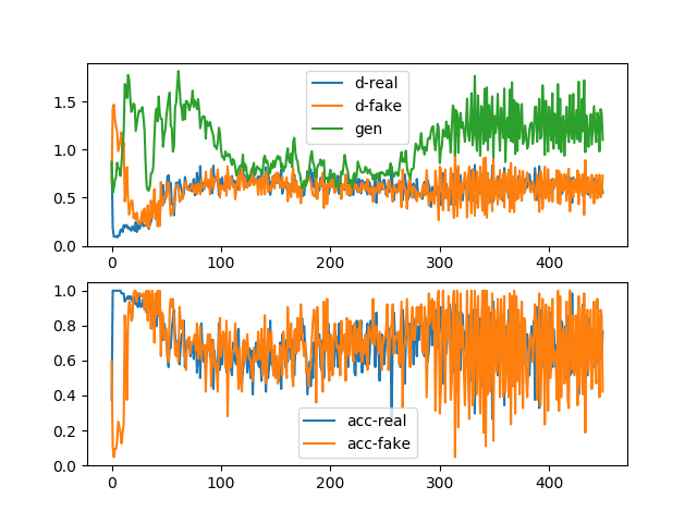
Line Plots of Loss and Accuracy for a Stable Generative Adversarial Network
Finally, we can review samples of generated images. Note: we are generating images using a reverse grayscale color map, meaning that the normal white figure on a background is inverted to a black figure on a white background. This was done to make the generated figures easier to review.
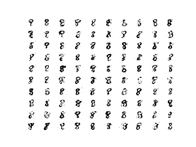
As we might expect, samples of images generated before epoch 100 are relatively poor in quality.
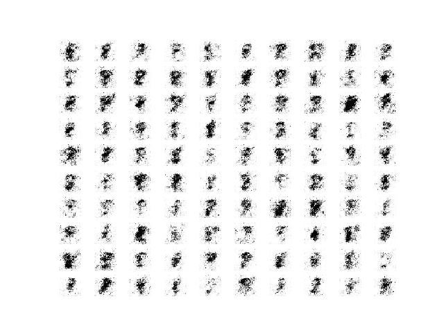
Sample of 100 Generated Images of a Handwritten Number 8 at Epoch 45 From a Stable GAN.
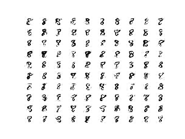
Samples of images generated between epochs 100 and 300 are plausible, and perhaps the best quality.
Sample of 100 Generated Images of a Handwritten Number 8 at Epoch 180 From a Stable GAN.
And samples of generated images after epoch 300 remain plausible, although perhaps have more noise, e.g. background noise.
Sample of 100 Generated Images of a Handwritten Number 8 at Epoch 450 From a Stable GAN.
These results are important, as it highlights that the quality generated can and does vary across the run, even after the training process becomes stable.
More training iterations, beyond some point of training stability may or may not result in higher quality images.
We can summarize these observations for stable GAN training as follows:
- Discriminator loss on real and fake images is expected to sit around 0.5.
- Generator loss on fake images is expected to sit between 0.5 and perhaps 2.0.
- Discriminator accuracy on real and fake images is expected to sit around 80%.
- Variance of generator and discriminator loss is expected to remain modest.
- The generator is expected to produce its highest quality images during a period of stability.
- Training stability may degenerate into periods of high-variance loss and corresponding lower quality generated images.
Now that we have a stable GAN model, we can look into modifying it to produce some specific failure cases.
There are two failure cases that are common to see when training GAN models on new problems; they are mode collapse and convergence failure.
How To Identify a Mode Collapse in a Generative Adversarial Network
A mode collapse refers to a generator model that is only capable of generating one or a small subset of different outcomes, or modes.
Here, mode refers to an output distribution, e.g. a multi-modal function refers to a function with more than one peak or optima. With a GAN generator model, a mode failure means that the vast number of points in the input latent space (e.g. hypersphere of 100 dimensions in many cases) result in one or a small subset of generated images.
Mode collapse, also known as the scenario, is a problem that occurs when the generator learns to map several different input z values to the same output point.
— NIPS 2016 Tutorial: Generative Adversarial Networks, 2016.
A mode collapse can be identified when reviewing a large sample of generated images. The images will show low diversity, with the same identical image or same small subset of identical images repeating many times.
A mode collapse can also be identified by reviewing the line plot of model loss. The line plot will show oscillations in the loss over time, most notably in the generator model, as the generator model is updated and jumps from generating one mode to another model that has different loss.
We can impair our stable GAN to suffer mode collapse a number of ways. Perhaps the most reliable is to restrict the size of the latent dimension directly, forcing the model to only generate a small subset of plausible outputs.
Specifically, the ‘latent_dim‘ variable can be changed from 100 to 1, and the experiment re-run.
# size of the latent space
latent_dim = 1
The full code listing is provided below for completeness.
# example of training an unstable gan for generating a handwritten digit
from os import makedirs
from numpy import expand_dims
from numpy import zeros
from numpy import ones
from numpy.random import randn
from numpy.random import randint
from keras.datasets.mnist import load_data
from keras.optimizers import Adam
from keras.models import Sequential
from keras.layers import Dense
from keras.layers import Reshape
from keras.layers import Flatten
from keras.layers import Conv2D
from keras.layers import Conv2DTranspose
from keras.layers import LeakyReLU
from keras.layers import BatchNormalization
from keras.initializers import RandomNormal
from matplotlib import pyplot

# define the standalone discriminator model
def define_discriminator(in_shape=(28,28,1)):
	# weight initialization
	init = RandomNormal(stddev=0.02)
	# define model
	model = Sequential()
	# downsample to 14x14
	model.add(Conv2D(64, (4,4), strides=(2,2), padding='same', kernel_initializer=init, input_shape=in_shape))
	model.add(BatchNormalization())
	model.add(LeakyReLU(alpha=0.2))
	# downsample to 7x7
	model.add(Conv2D(64, (4,4), strides=(2,2), padding='same', kernel_initializer=init))
	model.add(BatchNormalization())
	model.add(LeakyReLU(alpha=0.2))
	# classifier
	model.add(Flatten())
	model.add(Dense(1, activation='sigmoid'))
	# compile model
	opt = Adam(lr=0.0002, beta_1=0.5)
	model.compile(loss='binary_crossentropy', optimizer=opt, metrics=['accuracy'])
	return model

# define the standalone generator model
def define_generator(latent_dim):
	# weight initialization
	init = RandomNormal(stddev=0.02)
	# define model
	model = Sequential()
	# foundation for 7x7 image
	n_nodes = 128 * 7 * 7
	model.add(Dense(n_nodes, kernel_initializer=init, input_dim=latent_dim))
	model.add(LeakyReLU(alpha=0.2))
	model.add(Reshape((7, 7, 128)))
	# upsample to 14x14
	model.add(Conv2DTranspose(128, (4,4), strides=(2,2), padding='same', kernel_initializer=init))
	model.add(BatchNormalization())
	model.add(LeakyReLU(alpha=0.2))
	# upsample to 28x28
	model.add(Conv2DTranspose(128, (4,4), strides=(2,2), padding='same', kernel_initializer=init))
	model.add(BatchNormalization())
	model.add(LeakyReLU(alpha=0.2))
	# output 28x28x1
	model.add(Conv2D(1, (7,7), activation='tanh', padding='same', kernel_initializer=init))
	return model

# define the combined generator and discriminator model, for updating the generator
def define_gan(generator, discriminator):
	# make weights in the discriminator not trainable
	discriminator.trainable = False
	# connect them
	model = Sequential()
	# add generator
	model.add(generator)
	# add the discriminator
	model.add(discriminator)
	# compile model
	opt = Adam(lr=0.0002, beta_1=0.5)
	model.compile(loss='binary_crossentropy', optimizer=opt)
	return model

# load mnist images
def load_real_samples():
	# load dataset
	(trainX, trainy), (_, _) = load_data()
	# expand to 3d, e.g. add channels
	X = expand_dims(trainX, axis=-1)
	# select all of the examples for a given class
	selected_ix = trainy == 8
	X = X[selected_ix]
	# convert from ints to floats
	X = X.astype('float32')
	# scale from [0,255] to [-1,1]
	X = (X - 127.5) / 127.5
	return X

# # select real samples
def generate_real_samples(dataset, n_samples):
	# choose random instances
	ix = randint(0, dataset.shape[0], n_samples)
	# select images
	X = dataset[ix]
	# generate class labels
	y = ones((n_samples, 1))
	return X, y

# generate points in latent space as input for the generator
def generate_latent_points(latent_dim, n_samples):
	# generate points in the latent space
	x_input = randn(latent_dim * n_samples)
	# reshape into a batch of inputs for the network
	x_input = x_input.reshape(n_samples, latent_dim)
	return x_input

# use the generator to generate n fake examples, with class labels
def generate_fake_samples(generator, latent_dim, n_samples):
	# generate points in latent space
	x_input = generate_latent_points(latent_dim, n_samples)
	# predict outputs
	X = generator.predict(x_input)
	# create class labels
	y = zeros((n_samples, 1))
	return X, y

# generate samples and save as a plot and save the model
def summarize_performance(step, g_model, latent_dim, n_samples=100):
	# prepare fake examples
	X, _ = generate_fake_samples(g_model, latent_dim, n_samples)
	# scale from [-1,1] to [0,1]
	X = (X + 1) / 2.0
	# plot images
	for i in range(10 * 10):
		# define subplot
		pyplot.subplot(10, 10, 1 + i)
		# turn off axis
		pyplot.axis('off')
		# plot raw pixel data
		pyplot.imshow(X[i, :, :, 0], cmap='gray_r')
	# save plot to file
	pyplot.savefig('results_collapse/generated_plot_%03d.png' % (step+1))
	pyplot.close()
	# save the generator model
	g_model.save('results_collapse/model_%03d.h5' % (step+1))

# create a line plot of loss for the gan and save to file
def plot_history(d1_hist, d2_hist, g_hist, a1_hist, a2_hist):
	# plot loss
	pyplot.subplot(2, 1, 1)
	pyplot.plot(d1_hist, label='d-real')
	pyplot.plot(d2_hist, label='d-fake')
	pyplot.plot(g_hist, label='gen')
	pyplot.legend()
	# plot discriminator accuracy
	pyplot.subplot(2, 1, 2)
	pyplot.plot(a1_hist, label='acc-real')
	pyplot.plot(a2_hist, label='acc-fake')
	pyplot.legend()
	# save plot to file
	pyplot.savefig('results_collapse/plot_line_plot_loss.png')
	pyplot.close()

# train the generator and discriminator
def train(g_model, d_model, gan_model, dataset, latent_dim, n_epochs=10, n_batch=128):
	# calculate the number of batches per epoch
	bat_per_epo = int(dataset.shape[0] / n_batch)
	# calculate the total iterations based on batch and epoch
	n_steps = bat_per_epo * n_epochs
	# calculate the number of samples in half a batch
	half_batch = int(n_batch / 2)
	# prepare lists for storing stats each iteration
	d1_hist, d2_hist, g_hist, a1_hist, a2_hist = list(), list(), list(), list(), list()
	# manually enumerate epochs
	for i in range(n_steps):
		# get randomly selected 'real' samples
		X_real, y_real = generate_real_samples(dataset, half_batch)
		# update discriminator model weights
		d_loss1, d_acc1 = d_model.train_on_batch(X_real, y_real)
		# generate 'fake' examples
		X_fake, y_fake = generate_fake_samples(g_model, latent_dim, half_batch)
		# update discriminator model weights
		d_loss2, d_acc2 = d_model.train_on_batch(X_fake, y_fake)
		# prepare points in latent space as input for the generator
		X_gan = generate_latent_points(latent_dim, n_batch)
		# create inverted labels for the fake samples
		y_gan = ones((n_batch, 1))
		# update the generator via the discriminator's error
		g_loss = gan_model.train_on_batch(X_gan, y_gan)
		# summarize loss on this batch
		print('>%d, d1=%.3f, d2=%.3f g=%.3f, a1=%d, a2=%d' %
			(i+1, d_loss1, d_loss2, g_loss, int(100*d_acc1), int(100*d_acc2)))
		# record history
		d1_hist.append(d_loss1)
		d2_hist.append(d_loss2)
		g_hist.append(g_loss)
		a1_hist.append(d_acc1)
		a2_hist.append(d_acc2)
		# evaluate the model performance every 'epoch'
		if (i+1) % bat_per_epo == 0:
			summarize_performance(i, g_model, latent_dim)
	plot_history(d1_hist, d2_hist, g_hist, a1_hist, a2_hist)

# make folder for results
makedirs('results_collapse', exist_ok=True)
# size of the latent space
latent_dim = 1
# create the discriminator
discriminator = define_discriminator()
# create the generator
generator = define_generator(latent_dim)
# create the gan
gan_model = define_gan(generator, discriminator)
# load image data
dataset = load_real_samples()
print(dataset.shape)
# train model
train(generator, discriminator, gan_model, dataset, latent_dim)
Running the example will report the loss and accuracy each step of training, as before.
In this case, the loss for the discriminator sits in a sensible range, although the loss for the generator jumps up and down. The accuracy for the discriminator also shows higher values, many around 100%, meaning that for many batches, it has perfect skill at identifying real or fake examples, a bad sign for image quality or diversity.
>1, d1=0.963, d2=0.699 g=0.614, a1=28, a2=54
>2, d1=0.185, d2=5.084 g=0.097, a1=96, a2=0
>3, d1=0.088, d2=4.861 g=0.065, a1=100, a2=0
>4, d1=0.077, d2=4.202 g=0.090, a1=100, a2=0
>5, d1=0.062, d2=3.533 g=0.128, a1=100, a2=0
...
>446, d1=0.277, d2=0.261 g=0.684, a1=95, a2=100
>447, d1=0.201, d2=0.247 g=0.713, a1=96, a2=100
>448, d1=0.285, d2=0.285 g=0.728, a1=89, a2=100
>449, d1=0.351, d2=0.467 g=1.184, a1=92, a2=81
>450, d1=0.492, d2=0.388 g=1.351, a1=76, a2=100
The figure with learning curve and accuracy line plots is created and saved.
In the top subplot, we can see the loss for the generator (green) oscillating from sensible to high values over time, with a period of about 25 model updates (batches). We can also see some small oscillations in the loss for the discriminator on real and fake samples (orange and blue).
In the bottom subplot, we can see that the discriminator’s classification accuracy for identifying fake images remains high throughout the run. This suggests that the generator is poor at generating examples in some consistent way that makes it easy for the discriminator to identify the fake images.
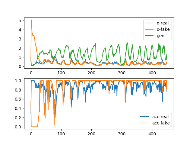
Line Plots of Loss and Accuracy for a Generative Adversarial Network With Mode Collapse
Reviewing generated images shows the expected feature of mode collapse, namely many identical generated examples, regardless of the input point in the latent space. It just so happens that we have changed the dimensionality of the latent space to be dramatically small to force this effect.
I have chosen an example of generated images that helps to make this clear. There appear to be only a few types of figure-eights in the image, one leaning left, one leaning right, and one sitting up with a blur.
I have drawn boxes around some of the similar examples in the image below to make this clearer.
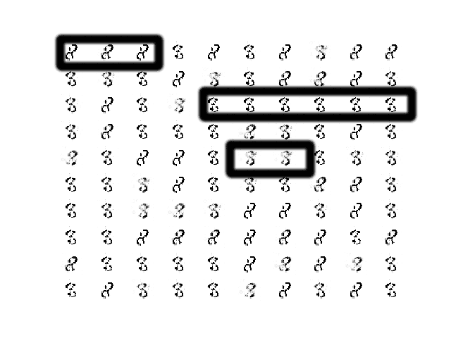
Sample of 100 Generated Images of a Handwritten Number 8 at Epoch 315 From a GAN That Has Suffered Mode Collapse.
A mode collapse is less common during training given the findings from the DCGAN model architecture and training configuration.
In summary, you can identify a mode collapse as follows:
- The loss for the generator, and probably the discriminator, is expected to oscillate over time.
- The generator model is expected to generate identical output images from different points in the latent space.
How To Identify Convergence Failure in a Generative Adversarial Network
Perhaps the most common failure when training a GAN is a failure to converge.
Typically, a neural network fails to converge when the model loss does not settle down during the training process. In the case of a GAN, a failure to converge refers to not finding an equilibrium between the discriminator and the generator.
The likely way that you will identify this type of failure is that the loss for the discriminator has gone to zero or close to zero. In some cases, the loss of the generator may also rise and continue to rise over the same period.
This type of loss is most commonly caused by the generator outputting garbage images that the discriminator can easily identify.
This type of failure might happen at the beginning of the run and continue throughout training, at which point you should halt the training process. For some unstable GANs, it is possible for the GAN to fall into this failure mode for a number of batch updates, or even a number of epochs, and then recover.
There are many ways to impair our stable GAN to achieve a convergence failure, such as changing one or both models to have insufficient capacity, changing the Adam optimization algorithm to be too aggressive, and using very large or very small kernel sizes in the models.
In this case, we will update the example to combine the real and fake samples when updating the discriminator. This simple change will cause the model to fail to converge.
This change is as simple as using the vstack() NumPy function to combine the real and fake samples and then calling the train_on_batch() function to update the discriminator model. The result is also a single loss and accuracy scores, meaning that the reporting of model performance, must also be updated.
The full code listing with these changes is provided below for completeness.
# example of training an unstable gan for generating a handwritten digit
from os import makedirs
from numpy import expand_dims
from numpy import zeros
from numpy import ones
from numpy import vstack
from numpy.random import randn
from numpy.random import randint
from keras.datasets.mnist import load_data
from keras.optimizers import Adam
from keras.models import Sequential
from keras.layers import Dense
from keras.layers import Reshape
from keras.layers import Flatten
from keras.layers import Conv2D
from keras.layers import Conv2DTranspose
from keras.layers import LeakyReLU
from keras.layers import BatchNormalization
from keras.initializers import RandomNormal
from matplotlib import pyplot

# define the standalone discriminator model
def define_discriminator(in_shape=(28,28,1)):
	# weight initialization
	init = RandomNormal(stddev=0.02)
	# define model
	model = Sequential()
	# downsample to 14x14
	model.add(Conv2D(64, (4,4), strides=(2,2), padding='same', kernel_initializer=init, input_shape=in_shape))
	model.add(BatchNormalization())
	model.add(LeakyReLU(alpha=0.2))
	# downsample to 7x7
	model.add(Conv2D(64, (4,4), strides=(2,2), padding='same', kernel_initializer=init))
	model.add(BatchNormalization())
	model.add(LeakyReLU(alpha=0.2))
	# classifier
	model.add(Flatten())
	model.add(Dense(1, activation='sigmoid'))
	# compile model
	opt = Adam(lr=0.0002, beta_1=0.5)
	model.compile(loss='binary_crossentropy', optimizer=opt, metrics=['accuracy'])
	return model

# define the standalone generator model
def define_generator(latent_dim):
	# weight initialization
	init = RandomNormal(stddev=0.02)
	# define model
	model = Sequential()
	# foundation for 7x7 image
	n_nodes = 128 * 7 * 7
	model.add(Dense(n_nodes, kernel_initializer=init, input_dim=latent_dim))
	model.add(LeakyReLU(alpha=0.2))
	model.add(Reshape((7, 7, 128)))
	# upsample to 14x14
	model.add(Conv2DTranspose(128, (4,4), strides=(2,2), padding='same', kernel_initializer=init))
	model.add(BatchNormalization())
	model.add(LeakyReLU(alpha=0.2))
	# upsample to 28x28
	model.add(Conv2DTranspose(128, (4,4), strides=(2,2), padding='same', kernel_initializer=init))
	model.add(BatchNormalization())
	model.add(LeakyReLU(alpha=0.2))
	# output 28x28x1
	model.add(Conv2D(1, (7,7), activation='tanh', padding='same', kernel_initializer=init))
	return model

# define the combined generator and discriminator model, for updating the generator
def define_gan(generator, discriminator):
	# make weights in the discriminator not trainable
	discriminator.trainable = False
	# connect them
	model = Sequential()
	# add generator
	model.add(generator)
	# add the discriminator
	model.add(discriminator)
	# compile model
	opt = Adam(lr=0.0002, beta_1=0.5)
	model.compile(loss='binary_crossentropy', optimizer=opt)
	return model

# load mnist images
def load_real_samples():
	# load dataset
	(trainX, trainy), (_, _) = load_data()
	# expand to 3d, e.g. add channels
	X = expand_dims(trainX, axis=-1)
	# select all of the examples for a given class
	selected_ix = trainy == 8
	X = X[selected_ix]
	# convert from ints to floats
	X = X.astype('float32')
	# scale from [0,255] to [-1,1]
	X = (X - 127.5) / 127.5
	return X

# # select real samples
def generate_real_samples(dataset, n_samples):
	# choose random instances
	ix = randint(0, dataset.shape[0], n_samples)
	# select images
	X = dataset[ix]
	# generate class labels
	y = ones((n_samples, 1))
	return X, y

# generate points in latent space as input for the generator
def generate_latent_points(latent_dim, n_samples):
	# generate points in the latent space
	x_input = randn(latent_dim * n_samples)
	# reshape into a batch of inputs for the network
	x_input = x_input.reshape(n_samples, latent_dim)
	return x_input

# use the generator to generate n fake examples, with class labels
def generate_fake_samples(generator, latent_dim, n_samples):
	# generate points in latent space
	x_input = generate_latent_points(latent_dim, n_samples)
	# predict outputs
	X = generator.predict(x_input)
	# create class labels
	y = zeros((n_samples, 1))
	return X, y

# generate samples and save as a plot and save the model
def summarize_performance(step, g_model, latent_dim, n_samples=100):
	# prepare fake examples
	X, _ = generate_fake_samples(g_model, latent_dim, n_samples)
	# scale from [-1,1] to [0,1]
	X = (X + 1) / 2.0
	# plot images
	for i in range(10 * 10):
		# define subplot
		pyplot.subplot(10, 10, 1 + i)
		# turn off axis
		pyplot.axis('off')
		# plot raw pixel data
		pyplot.imshow(X[i, :, :, 0], cmap='gray_r')
	# save plot to file
	pyplot.savefig('results_convergence/generated_plot_%03d.png' % (step+1))
	pyplot.close()
	# save the generator model
	g_model.save('results_convergence/model_%03d.h5' % (step+1))

# create a line plot of loss for the gan and save to file
def plot_history(d_hist, g_hist, a_hist):
	# plot loss
	pyplot.subplot(2, 1, 1)
	pyplot.plot(d_hist, label='dis')
	pyplot.plot(g_hist, label='gen')
	pyplot.legend()
	# plot discriminator accuracy
	pyplot.subplot(2, 1, 2)
	pyplot.plot(a_hist, label='acc')
	pyplot.legend()
	# save plot to file
	pyplot.savefig('results_convergence/plot_line_plot_loss.png')
	pyplot.close()

# train the generator and discriminator
def train(g_model, d_model, gan_model, dataset, latent_dim, n_epochs=10, n_batch=128):
	# calculate the number of batches per epoch
	bat_per_epo = int(dataset.shape[0] / n_batch)
	# calculate the total iterations based on batch and epoch
	n_steps = bat_per_epo * n_epochs
	# calculate the number of samples in half a batch
	half_batch = int(n_batch / 2)
	# prepare lists for storing stats each iteration
	d_hist, g_hist, a_hist = list(), list(), list()
	# manually enumerate epochs
	for i in range(n_steps):
		# get randomly selected 'real' samples
		X_real, y_real = generate_real_samples(dataset, half_batch)
		# generate 'fake' examples
		X_fake, y_fake = generate_fake_samples(g_model, latent_dim, half_batch)
		# combine into one batch
		X, y = vstack((X_real, X_fake)), vstack((y_real, y_fake))
		# update discriminator model weights
		d_loss, d_acc = d_model.train_on_batch(X, y)
		# prepare points in latent space as input for the generator
		X_gan = generate_latent_points(latent_dim, n_batch)
		# create inverted labels for the fake samples
		y_gan = ones((n_batch, 1))
		# update the generator via the discriminator's error
		g_loss = gan_model.train_on_batch(X_gan, y_gan)
		# summarize loss on this batch
		print('>%d, d=%.3f, g=%.3f, a=%d' % (i+1, d_loss, g_loss, int(100*d_acc)))
		# record history
		d_hist.append(d_loss)
		g_hist.append(g_loss)
		a_hist.append(d_acc)
		# evaluate the model performance every 'epoch'
		if (i+1) % bat_per_epo == 0:
			summarize_performance(i, g_model, latent_dim)
	plot_history(d_hist, g_hist, a_hist)

# make folder for results
makedirs('results_convergence', exist_ok=True)
# size of the latent space
latent_dim = 50
# create the discriminator
discriminator = define_discriminator()
# create the generator
generator = define_generator(latent_dim)
# create the gan
gan_model = define_gan(generator, discriminator)
# load image data
dataset = load_real_samples()
print(dataset.shape)
# train model
train(generator, discriminator, gan_model, dataset, latent_dim)
Running the example reports loss and accuracy for each model update.
A clear sign of this type of failure is the rapid drop of the discriminator loss towards zero, where it remains.
This is what we see in this case.
>1, d=0.514, g=0.969, a=80
>2, d=0.475, g=0.395, a=74
>3, d=0.452, g=0.223, a=69
>4, d=0.302, g=0.220, a=85
>5, d=0.177, g=0.195, a=100
>6, d=0.122, g=0.200, a=100
>7, d=0.088, g=0.179, a=100
>8, d=0.075, g=0.159, a=100
>9, d=0.071, g=0.167, a=100
>10, d=0.102, g=0.127, a=100
...
>446, d=0.000, g=0.001, a=100
>447, d=0.000, g=0.001, a=100
>448, d=0.000, g=0.001, a=100
>449, d=0.000, g=0.001, a=100
>450, d=0.000, g=0.001, a=100
Line plots of learning curves and classification accuracy are created.
The top subplot shows the loss for the discriminator (blue) and generator (orange) and clearly shows the drop of both values down towards zero over the first 20 to 30 iterations, where it remains for the rest of the run.
The bottom subplot shows the discriminator classification accuracy sitting on 100% for the same period, meaning the model is perfect at identifying real and fake images. The expectation is that there is something about fake images that makes them very easy for the discriminator to identify.
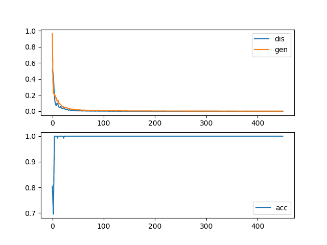
Line Plots of Loss and Accuracy for a Generative Adversarial Network With a Convergence Failure
Finally, reviewing samples of generated images makes it clear why the discriminator is so successful.
Samples of images generated at each epoch are all very low quality, showing static, perhaps with a faint figure eight in the background.
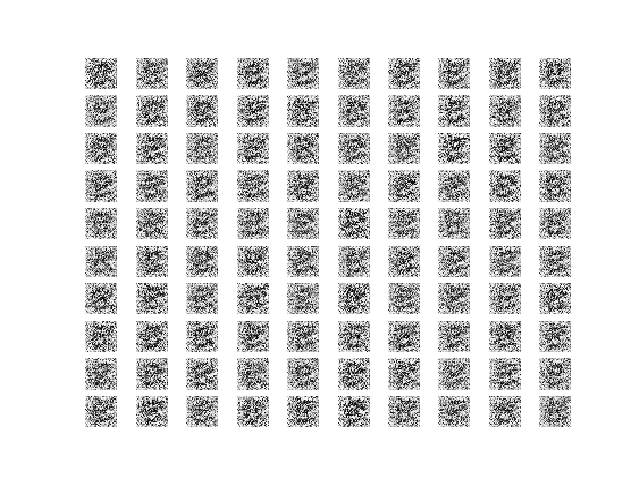
Sample of 100 Generated Images of a Handwritten Number 8 at Epoch 450 From a GAN That Has a Convergence Failure via Combined Updates to the Discriminator.
It is useful to see another example of this type of failure.
In this case, the configuration of the Adam optimization algorithm can be modified to use the defaults, which in turn makes the updates to the models aggressive and causes a failure for the training process to find a point of equilibrium between training the two models.
For example, the discriminator can be compiled as follows:
...
# compile model
model.compile(loss='binary_crossentropy', optimizer='adam', metrics=['accuracy'])
And the composite GAN model can be compiled as follows:
...
# compile model
model.compile(loss='binary_crossentropy', optimizer='adam')
The full code listing is provided below for completeness.
# example of training an unstable gan for generating a handwritten digit
from os import makedirs
from numpy import expand_dims
from numpy import zeros
from numpy import ones
from numpy.random import randn
from numpy.random import randint
from keras.datasets.mnist import load_data
from keras.models import Sequential
from keras.layers import Dense
from keras.layers import Reshape
from keras.layers import Flatten
from keras.layers import Conv2D
from keras.layers import Conv2DTranspose
from keras.layers import LeakyReLU
from keras.layers import BatchNormalization
from keras.initializers import RandomNormal
from matplotlib import pyplot

# define the standalone discriminator model
def define_discriminator(in_shape=(28,28,1)):
	# weight initialization
	init = RandomNormal(stddev=0.02)
	# define model
	model = Sequential()
	# downsample to 14x14
	model.add(Conv2D(64, (4,4), strides=(2,2), padding='same', kernel_initializer=init, input_shape=in_shape))
	model.add(BatchNormalization())
	model.add(LeakyReLU(alpha=0.2))
	# downsample to 7x7
	model.add(Conv2D(64, (4,4), strides=(2,2), padding='same', kernel_initializer=init))
	model.add(BatchNormalization())
	model.add(LeakyReLU(alpha=0.2))
	# classifier
	model.add(Flatten())
	model.add(Dense(1, activation='sigmoid'))
	# compile model
	model.compile(loss='binary_crossentropy', optimizer='adam', metrics=['accuracy'])
	return model

# define the standalone generator model
def define_generator(latent_dim):
	# weight initialization
	init = RandomNormal(stddev=0.02)
	# define model
	model = Sequential()
	# foundation for 7x7 image
	n_nodes = 128 * 7 * 7
	model.add(Dense(n_nodes, kernel_initializer=init, input_dim=latent_dim))
	model.add(LeakyReLU(alpha=0.2))
	model.add(Reshape((7, 7, 128)))
	# upsample to 14x14
	model.add(Conv2DTranspose(128, (4,4), strides=(2,2), padding='same', kernel_initializer=init))
	model.add(BatchNormalization())
	model.add(LeakyReLU(alpha=0.2))
	# upsample to 28x28
	model.add(Conv2DTranspose(128, (4,4), strides=(2,2), padding='same', kernel_initializer=init))
	model.add(BatchNormalization())
	model.add(LeakyReLU(alpha=0.2))
	# output 28x28x1
	model.add(Conv2D(1, (7,7), activation='tanh', padding='same', kernel_initializer=init))
	return model

# define the combined generator and discriminator model, for updating the generator
def define_gan(generator, discriminator):
	# make weights in the discriminator not trainable
	discriminator.trainable = False
	# connect them
	model = Sequential()
	# add generator
	model.add(generator)
	# add the discriminator
	model.add(discriminator)
	# compile model
	model.compile(loss='binary_crossentropy', optimizer='adam')
	return model

# load mnist images
def load_real_samples():
	# load dataset
	(trainX, trainy), (_, _) = load_data()
	# expand to 3d, e.g. add channels
	X = expand_dims(trainX, axis=-1)
	# select all of the examples for a given class
	selected_ix = trainy == 8
	X = X[selected_ix]
	# convert from ints to floats
	X = X.astype('float32')
	# scale from [0,255] to [-1,1]
	X = (X - 127.5) / 127.5
	return X

# select real samples
def generate_real_samples(dataset, n_samples):
	# choose random instances
	ix = randint(0, dataset.shape[0], n_samples)
	# select images
	X = dataset[ix]
	# generate class labels
	y = ones((n_samples, 1))
	return X, y

# generate points in latent space as input for the generator
def generate_latent_points(latent_dim, n_samples):
	# generate points in the latent space
	x_input = randn(latent_dim * n_samples)
	# reshape into a batch of inputs for the network
	x_input = x_input.reshape(n_samples, latent_dim)
	return x_input

# use the generator to generate n fake examples, with class labels
def generate_fake_samples(generator, latent_dim, n_samples):
	# generate points in latent space
	x_input = generate_latent_points(latent_dim, n_samples)
	# predict outputs
	X = generator.predict(x_input)
	# create class labels
	y = zeros((n_samples, 1))
	return X, y

# generate samples and save as a plot and save the model
def summarize_performance(step, g_model, latent_dim, n_samples=100):
	# prepare fake examples
	X, _ = generate_fake_samples(g_model, latent_dim, n_samples)
	# scale from [-1,1] to [0,1]
	X = (X + 1) / 2.0
	# plot images
	for i in range(10 * 10):
		# define subplot
		pyplot.subplot(10, 10, 1 + i)
		# turn off axis
		pyplot.axis('off')
		# plot raw pixel data
		pyplot.imshow(X[i, :, :, 0], cmap='gray_r')
	# save plot to file
	pyplot.savefig('results_opt/generated_plot_%03d.png' % (step+1))
	pyplot.close()
	# save the generator model
	g_model.save('results_opt/model_%03d.h5' % (step+1))

# create a line plot of loss for the gan and save to file
def plot_history(d1_hist, d2_hist, g_hist, a1_hist, a2_hist):
	# plot loss
	pyplot.subplot(2, 1, 1)
	pyplot.plot(d1_hist, label='d-real')
	pyplot.plot(d2_hist, label='d-fake')
	pyplot.plot(g_hist, label='gen')
	pyplot.legend()
	# plot discriminator accuracy
	pyplot.subplot(2, 1, 2)
	pyplot.plot(a1_hist, label='acc-real')
	pyplot.plot(a2_hist, label='acc-fake')
	pyplot.legend()
	# save plot to file
	pyplot.savefig('results_opt/plot_line_plot_loss.png')
	pyplot.close()

# train the generator and discriminator
def train(g_model, d_model, gan_model, dataset, latent_dim, n_epochs=10, n_batch=128):
	# calculate the number of batches per epoch
	bat_per_epo = int(dataset.shape[0] / n_batch)
	# calculate the total iterations based on batch and epoch
	n_steps = bat_per_epo * n_epochs
	# calculate the number of samples in half a batch
	half_batch = int(n_batch / 2)
	# prepare lists for storing stats each iteration
	d1_hist, d2_hist, g_hist, a1_hist, a2_hist = list(), list(), list(), list(), list()
	# manually enumerate epochs
	for i in range(n_steps):
		# get randomly selected 'real' samples
		X_real, y_real = generate_real_samples(dataset, half_batch)
		# update discriminator model weights
		d_loss1, d_acc1 = d_model.train_on_batch(X_real, y_real)
		# generate 'fake' examples
		X_fake, y_fake = generate_fake_samples(g_model, latent_dim, half_batch)
		# update discriminator model weights
		d_loss2, d_acc2 = d_model.train_on_batch(X_fake, y_fake)
		# prepare points in latent space as input for the generator
		X_gan = generate_latent_points(latent_dim, n_batch)
		# create inverted labels for the fake samples
		y_gan = ones((n_batch, 1))
		# update the generator via the discriminator's error
		g_loss = gan_model.train_on_batch(X_gan, y_gan)
		# summarize loss on this batch
		print('>%d, d1=%.3f, d2=%.3f g=%.3f, a1=%d, a2=%d' %
			(i+1, d_loss1, d_loss2, g_loss, int(100*d_acc1), int(100*d_acc2)))
		# record history
		d1_hist.append(d_loss1)
		d2_hist.append(d_loss2)
		g_hist.append(g_loss)
		a1_hist.append(d_acc1)
		a2_hist.append(d_acc2)
		# evaluate the model performance every 'epoch'
		if (i+1) % bat_per_epo == 0:
			summarize_performance(i, g_model, latent_dim)
	plot_history(d1_hist, d2_hist, g_hist, a1_hist, a2_hist)

# make folder for results
makedirs('results_opt', exist_ok=True)
# size of the latent space
latent_dim = 50
# create the discriminator
discriminator = define_discriminator()
# create the generator
generator = define_generator(latent_dim)
# create the gan
gan_model = define_gan(generator, discriminator)
# load image data
dataset = load_real_samples()
print(dataset.shape)
# train model
train(generator, discriminator, gan_model, dataset, latent_dim)
Running the example reports the loss and accuracy for each step during training, as before.
As we expected, the loss for the discriminator rapidly falls to a value close to zero, where it remains, and classification accuracy for the discriminator on real and fake examples remains at 100%.
>1, d1=0.728, d2=0.902 g=0.763, a1=54, a2=12
>2, d1=0.001, d2=4.509 g=0.033, a1=100, a2=0
>3, d1=0.000, d2=0.486 g=0.542, a1=100, a2=76
>4, d1=0.000, d2=0.446 g=0.733, a1=100, a2=82
>5, d1=0.002, d2=0.855 g=0.649, a1=100, a2=46
...
>446, d1=0.000, d2=0.000 g=10.410, a1=100, a2=100
>447, d1=0.000, d2=0.000 g=10.414, a1=100, a2=100
>448, d1=0.000, d2=0.000 g=10.419, a1=100, a2=100
>449, d1=0.000, d2=0.000 g=10.424, a1=100, a2=100
>450, d1=0.000, d2=0.000 g=10.427, a1=100, a2=100
A plot of the learning curves and accuracy from training the model with this single change is created.
The plot shows that this change causes the loss for the discriminator to crash down to a value close to zero and remain there. An important difference for this case is that the loss for the generator rises quickly and continues to rise for the duration of training.
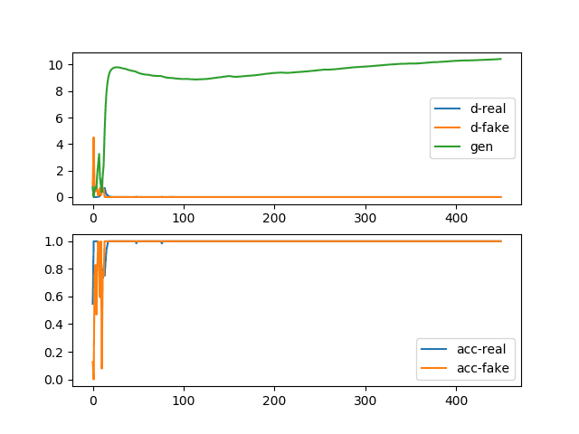
Sample of 100 Generated Images of a Handwritten Number 8 at Epoch 450 From a GAN That Has a Convergence Failure via Aggressive Optimization.
We can review the properties of a convergence failure as follows:
- The loss for the discriminator is expected to rapidly decrease to a value close to zero where it remains during training.
- The loss for the generator is expected to either decrease to zero or continually decrease during training.
- The generator is expected to produce extremely low-quality images that are easily identified as fake by the discriminator.
Further Reading
This section provides more resources on the topic if you are looking to go deeper.
Papers
- Generative Adversarial Networks, 2014.
- Tutorial: Generative Adversarial Networks, NIPS, 2016.
- Unsupervised Representation Learning with Deep Convolutional Generative Adversarial Networks, 2015.
Articles
Summary
In this tutorial, you discovered how to identify stable and unstable GAN training by reviewing examples of generated images and plots of metrics recorded during training.
Specifically, you learned:
- How to identify a stable GAN training process from the generator and discriminator loss over time.
- How to identify a mode collapse by reviewing both learning curves and generated images.
- How to identify a convergence failure by reviewing learning curves of generator and discriminator loss over time.
Do you have any questions?
Ask your questions in the comments below and I will do my best to answer.
The post How to Identify and Diagnose GAN Failure Modes appeared first on Machine Learning Mastery.