
Author: Jason Brownlee
The Generative Adversarial Network, or GAN for short, is an architecture for training a generative model.
The architecture is comprised of two models. The generator that we are interested in, and a discriminator model that is used to assist in the training of the generator. Initially, both of the generator and discriminator models were implemented as Multilayer Perceptrons (MLP), although more recently, the models are implemented as deep convolutional neural networks.
It can be challenging to understand how a GAN is trained and exactly how to understand and implement the loss function for the generator and discriminator models.
In this tutorial, you will discover how to implement the generative adversarial network training algorithm and loss functions.
After completing this tutorial, you will know:
- How to implement the training algorithm for a generative adversarial network.
- How the loss function for the discriminator and generator work.
- How to implement weight updates for the discriminator and generator models in practice.
Discover how to develop DCGANs, conditional GANs, Pix2Pix, CycleGANs, and more with Keras in my new GANs book, with 29 step-by-step tutorials and full source code.
Let’s get started.

How to Code the Generative Adversarial Network Training Algorithm and Loss Functions
Photo by Hilary Charlotte, some rights reserved.
Tutorial Overview
This tutorial is divided into three parts; they are:
- How to Implement the GAN Training Algorithm
- Understanding the GAN Loss Function
- How to Train GAN Models in Practice
Note: The code examples in this tutorial are snippets only, not standalone runnable examples. They are designed to help you develop an intuition for the algorithm and they can be used as the starting point for implementing the GAN training algorithm on your own project.
How to Implement the GAN Training Algorithm
The GAN training algorithm involves training both the discriminator and the generator model in parallel.
The algorithm is summarized in the figure below, taken from the original 2014 paper by Goodfellow, et al. titled “Generative Adversarial Networks.”
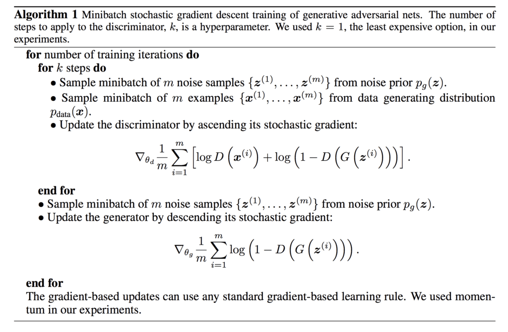
Summary of the Generative Adversarial Network Training Algorithm.Taken from: Generative Adversarial Networks.
Let’s take some time to unpack and get comfortable with this algorithm.
The outer loop of the algorithm involves iterating over steps to train the models in the architecture. One cycle through this loop is not an epoch: it is a single update comprised of specific batch updates to the discriminator and generator models.
An epoch is defined as one cycle through a training dataset, where the samples in a training dataset are used to update the model weights in mini-batches. For example, a training dataset of 100 samples used to train a model with a mini-batch size of 10 samples would involve 10 mini batch updates per epoch. The model would be fit for a given number of epochs, such as 500.
This is often hidden from you via the automated training of a model via a call to the fit() function and specifying the number of epochs and the size of each mini-batch.
In the case of the GAN, the number of training iterations must be defined based on the size of your training dataset and batch size. In the case of a dataset with 100 samples, a batch size of 10, and 500 training epochs, we would first calculate the number of batches per epoch and use this to calculate the total number of training iterations using the number of epochs.
For example:
...
batches_per_epoch = floor(dataset_size / batch_size)
total_iterations = batches_per_epoch * total_epochs
In the case of a dataset of 500 samples, a batch size of 10, and 500 epochs, the GAN would be trained for floor(100 / 10) * 500 or 5,000 total iterations.
Next, we can see that one iteration of training results in possibly multiple updates to the discriminator and one update to the generator, where the number of updates to the discriminator is a hyperparameter that is set to 1.
The training process consists of simultaneous SGD. On each step, two minibatches are sampled: a minibatch of x values from the dataset and a minibatch of z values drawn from the model’s prior over latent variables. Then two gradient steps are made simultaneously …
— NIPS 2016 Tutorial: Generative Adversarial Networks, 2016.
We can therefore summarize the training algorithm with Python pseudocode as follows:
# gan training algorithm
def train_gan(dataset, n_epochs, n_batch):
	# calculate the number of batches per epoch
	batches_per_epoch = int(len(dataset) / n_batch)
	# calculate the number of training iterations
	n_steps = batches_per_epoch * n_epochs
	# gan training algorithm
	for i in range(n_steps):
		# update the discriminator model
		# ...
		# update the generator model
		# ...
An alternative approach may involve enumerating the number of training epochs and splitting the training dataset into batches for each epoch.
Updating the discriminator model involves a few steps.
First, a batch of random points from the latent space must be selected for use as input to the generator model to provide the basis for the generated or ‘fake‘ samples. Then a batch of samples from the training dataset must be selected for input to the discriminator as the ‘real‘ samples.
Next, the discriminator model must make predictions for the real and fake samples and the weights of the discriminator must be updated proportional to how correct or incorrect those predictions were. The predictions are probabilities and we will get into the nature of the predictions and the loss function that is minimized in the next section. For now, we can outline what these steps actually look like in practice.
We need a generator and a discriminator model, e.g. such as a Keras model. These can be provided as arguments to the training function.
Next, we must generate points from the latent space and then use the generator model in its current form to generate some fake images. For example:
...
# generate points in the latent space
z = randn(latent_dim * n_batch)
# reshape into a batch of inputs for the network
z = x_input.reshape(n_batch, latent_dim)
# generate fake images
fake = generator.predict(x_input)
Note that the size of the latent dimension is also provided as a hyperparameter to the training algorithm.
We then must select a batch of real samples, and this too will be wrapped into a function.
...
# select a batch of random real images
ix = randint(0, len(dataset), n_batch)
# retrieve real images
real = dataset[ix]
The discriminator model must then make a prediction for each of the generated and real images and the weights must be updated.
# gan training algorithm
def train_gan(generator, discriminator, dataset, latent_dim, n_epochs, n_batch):
	# calculate the number of batches per epoch
	batches_per_epoch = int(len(dataset) / n_batch)
	# calculate the number of training iterations
	n_steps = batches_per_epoch * n_epochs
	# gan training algorithm
	for i in range(n_steps):
		# generate points in the latent space
		z = randn(latent_dim * n_batch)
		# reshape into a batch of inputs for the network
		z = z.reshape(n_batch, latent_dim)
		# generate fake images
		fake = generator.predict(z)
		# select a batch of random real images
		ix = randint(0, len(dataset), n_batch)
		# retrieve real images
		real = dataset[ix]
		# update weights of the discriminator model
		# ...

		# update the generator model
		# ...
Next, the generator model must be updated.
Again, a batch of random points from the latent space must be selected and passed to the generator to generate fake images, and then passed to the discriminator to classify.
...
# generate points in the latent space
z = randn(latent_dim * n_batch)
# reshape into a batch of inputs for the network
z = z.reshape(n_batch, latent_dim)
# generate fake images
fake = generator.predict(z)
# classify as real or fake
result = discriminator.predict(fake)
The response can then be used to update the weights of the generator model.
# gan training algorithm
def train_gan(generator, discriminator, dataset, latent_dim, n_epochs, n_batch):
	# calculate the number of batches per epoch
	batches_per_epoch = int(len(dataset) / n_batch)
	# calculate the number of training iterations
	n_steps = batches_per_epoch * n_epochs
	# gan training algorithm
	for i in range(n_steps):
		# generate points in the latent space
		z = randn(latent_dim * n_batch)
		# reshape into a batch of inputs for the network
		z = z.reshape(n_batch, latent_dim)
		# generate fake images
		fake = generator.predict(z)
		# select a batch of random real images
		ix = randint(0, len(dataset), n_batch)
		# retrieve real images
		real = dataset[ix]
		# update weights of the discriminator model
		# ...
		# generate points in the latent space
		z = randn(latent_dim * n_batch)
		# reshape into a batch of inputs for the network
		z = z.reshape(n_batch, latent_dim)
		# generate fake images
		fake = generator.predict(z)
		# classify as real or fake
		result = discriminator.predict(fake)
		# update weights of the generator model
		# ...
It is interesting that the discriminator is updated with two batches of samples each training iteration whereas the generator is only updated with a single batch of samples per training iteration.
Now that we have defined the training algorithm for the GAN, we need to understand how the model weights are updated. This requires understanding the loss function used to train the GAN.
Want to Develop GANs from Scratch?
Take my free 7-day email crash course now (with sample code).
Click to sign-up and also get a free PDF Ebook version of the course.
Understanding the GAN Loss Function
The discriminator is trained to correctly classify real and fake images.
This is achieved by maximizing the log of predicted probability of real images and the log of the inverted probability of fake images, averaged over each mini-batch of examples.
Recall that we add log probabilities, which is the same as multiplying probabilities, although without vanishing into small numbers. Therefore, we can understand this loss function as seeking probabilities close to 1.0 for real images and probabilities close to 0.0 for fake images, inverted to become larger numbers. The addition of these values means that lower average values of this loss function result in better performance of the discriminator.
Inverting this to a minimization problem, it should not be surprising if you are familiar with developing neural networks for binary classification, as this is exactly the approach used.
This is just the standard cross-entropy cost that is minimized when training a standard binary classifier with a sigmoid output. The only difference is that the classifier is trained on two minibatches of data; one coming from the dataset, where the label is 1 for all examples, and one coming from the generator, where the label is 0 for all examples.
— NIPS 2016 Tutorial: Generative Adversarial Networks, 2016.
The generator is more tricky.
The GAN algorithm defines the generator model’s loss as minimizing the log of the inverted probability of the discriminator’s prediction of fake images, averaged over a mini-batch.
This is straightforward, but according to the authors, it is not effective in practice when the generator is poor and the discriminator is good at rejecting fake images with high confidence. The loss function no longer gives good gradient information that the generator can use to adjust weights and instead saturates.
In this case, log(1 − D(G(z))) saturates. Rather than training G to minimize log(1 − D(G(z))) we can train G to maximize log D(G(z)). This objective function results in the same fixed point of the dynamics of G and D but provides much stronger gradients early in learning.
— Generative Adversarial Networks, 2014.
Instead, the authors recommend maximizing the log of the discriminator’s predicted probability for fake images.
The change is subtle.
In the first case, the generator is trained to minimize the probability of the discriminator being correct. With this change to the loss function, the generator is trained to maximize the probability of the discriminator being incorrect.
In the minimax game, the generator minimizes the log-probability of the discriminator being correct. In this game, the generator maximizes the log probability of the discriminator being mistaken.
— NIPS 2016 Tutorial: Generative Adversarial Networks, 2016.
The sign of this loss function can then be inverted to give a familiar minimizing loss function for training the generator. As such, this is sometimes referred to as the -log D trick for training GANs.
Our baseline comparison is DCGAN, a GAN with a convolutional architecture trained with the standard GAN procedure using the −log D trick.
— Wasserstein GAN, 2017.
Now that we understand the GAN loss function, we can look at how the discriminator and the generator model can be updated in practice.
How to Train GAN Models in Practice
The practical implementation of the GAN loss function and model updates is straightforward.
We will look at examples using the Keras library.
We can implement the discriminator directly by configuring the discriminator model to predict a probability of 1 for real images and 0 for fake images and minimizing the cross-entropy loss, specifically the binary cross-entropy loss.
For example, a snippet of our model definition with Keras for the discriminator might look as follows for the output layer and the compilation of the model with the appropriate loss function.
...
# output layer
model.add(Dense(1, activation='sigmoid'))
# compile model
model.compile(loss='binary_crossentropy', ...)
The defined model can be trained for each batch of real and fake samples providing arrays of 1s and 0s for the expected outcome.
The ones() and zeros() NumPy functions can be used to create these target labels, and the Keras function train_on_batch() can be used to update the model for each batch of samples.
...
X_fake = ...
X_real = ...
# define target labels for fake images
y_fake = zeros((n_batch, 1))
# update the discriminator for fake images
discriminator.train_on_batch(X_fake, y_fake)
# define target labels for real images
y_real = ones((n_batch, 1))
# update the discriminator for real images
discriminator.train_on_batch(X_real, y_real)
The discriminator model will be trained to predict the probability of “realness” of a given input image that can be interpreted as a class label of class=0 for fake and class=1 for real.
The generator is trained to maximize the discriminator predicting a high probability of “realness” for generated images.
This is achieved by updating the generator via the discriminator with the class label of 1 for the generated images. The discriminator is not updated in this operation but provides the gradient information required to update the weights of the generator model.
For example, if the discriminator predicts a low average probability for the batch of generated images, then this will result in a large error signal propagated backward into the generator given the “expected probability” for the samples was 1.0 for real. This large error signal, in turn, results in relatively large changes to the generator to hopefully improve its ability at generating fake samples on the next batch.
This can be implemented in Keras by creating a composite model that combines the generator and discriminator models, allowing the output images from the generator to flow into discriminator directly, and in turn, allow the error signals from the predicted probabilities of the discriminator to flow back through the weights of the generator model.
For example:
# define a composite gan model for the generator and discriminator
def define_gan(generator, discriminator):
	# make weights in the discriminator not trainable
	discriminator.trainable = False
	# connect them
	model = Sequential()
	# add generator
	model.add(generator)
	# add the discriminator
	model.add(discriminator)
	# compile model
	model.compile(loss='binary_crossentropy', optimizer='adam')
	return model
The composite model can then be updated using fake images and real class labels.
...
# generate points in the latent space
z = randn(latent_dim * n_batch)
# reshape into a batch of inputs for the network
z = z.reshape(n_batch, latent_dim)
# define target labels for real images
y_real = ones((n_batch, 1))
# update generator model
gan_model.train_on_batch(z, y_real)
That completes out tour of the GAN training algorithm, loss function and weight update details for the discriminator and generator models.
Further Reading
This section provides more resources on the topic if you are looking to go deeper.
Papers
- Generative Adversarial Networks, 2014.
- NIPS 2016 Tutorial: Generative Adversarial Networks, 2016.
- Wasserstein GAN, 2017.
Articles
Summary
In this tutorial, you discovered how to implement the generative adversarial network training algorithm and loss functions.
Specifically, you learned:
- How to implement the training algorithm for a generative adversarial network.
- How the loss function for the discriminator and generator work.
- How to implement weight updates for the discriminator and generator models in practice.
Do you have any questions?
Ask your questions in the comments below and I will do my best to answer.
The post How to Code the GAN Training Algorithm and Loss Functions appeared first on Machine Learning Mastery.