
Author: Jason Brownlee
The Pix2Pix GAN is a generator model for performing image-to-image translation trained on paired examples.
For example, the model can be used to translate images of daytime to nighttime, or from sketches of products like shoes to photographs of products.
The benefit of the Pix2Pix model is that compared to other GANs for conditional image generation, it is relatively simple and capable of generating large high-quality images across a variety of image translation tasks.
The model is very impressive but has an architecture that appears somewhat complicated to implement for beginners.
In this tutorial, you will discover how to implement the Pix2Pix GAN architecture from scratch using the Keras deep learning framework.
After completing this tutorial, you will know:
- How to develop the PatchGAN discriminator model for the Pix2Pix GAN.
- How to develop the U-Net encoder-decoder generator model for the Pix2Pix GAN.
- How to implement the composite model for updating the generator and how to train both models.
Discover how to develop DCGANs, conditional GANs, Pix2Pix, CycleGANs, and more with Keras in my new GANs book, with 29 step-by-step tutorials and full source code.
Let’s get started.

How to Implement Pix2Pix GAN Models From Scratch With Keras
Photo by Ray in Manila, some rights reserved.
Tutorial Overview
This tutorial is divided into five parts; they are:
- What Is the Pix2Pix GAN?
- How to Implement the PatchGAN Discriminator Model
- How to Implement the U-Net Generator Model
- How to Implement Adversarial and L1 Loss
- How to Update Model Weights
What Is the Pix2Pix GAN?
Pix2Pix is a Generative Adversarial Network, or GAN, model designed for general purpose image-to-image translation.
The approach was presented by Phillip Isola, et al. in their 2016 paper titled “Image-to-Image Translation with Conditional Adversarial Networks” and presented at CVPR in 2017.
The GAN architecture is comprised of a generator model for outputting new plausible synthetic images and a discriminator model that classifies images as real (from the dataset) or fake (generated). The discriminator model is updated directly, whereas the generator model is updated via the discriminator model. As such, the two models are trained simultaneously in an adversarial process where the generator seeks to better fool the discriminator and the discriminator seeks to better identify the counterfeit images.
The Pix2Pix model is a type of conditional GAN, or cGAN, where the generation of the output image is conditional on an input, in this case, a source image. The discriminator is provided both with a source image and the target image and must determine whether the target is a plausible transformation of the source image.
Again, the discriminator model is updated directly, and the generator model is updated via the discriminator model, although the loss function is updated. The generator is trained via adversarial loss, which encourages the generator to generate plausible images in the target domain. The generator is also updated via L1 loss measured between the generated image and the expected output image. This additional loss encourages the generator model to create plausible translations of the source image.
The Pix2Pix GAN has been demonstrated on a range of image-to-image translation tasks such as converting maps to satellite photographs, black and white photographs to color, and sketches of products to product photographs.
Now that we are familiar with the Pix2Pix GAN, let’s explore how we can implement it using the Keras deep learning library.
Want to Develop GANs from Scratch?
Take my free 7-day email crash course now (with sample code).
Click to sign-up and also get a free PDF Ebook version of the course.
How to Implement the PatchGAN Discriminator Model
The discriminator model in the Pix2Pix GAN is implemented as a PatchGAN.
The PatchGAN is designed based on the size of the receptive field, sometimes called the effective receptive field. The receptive field is the relationship between one output activation of the model to an area on the input image (actually volume as it proceeded down the input channels).
A PatchGAN with the size 70×70 is used, which means that the output (or each output) of the model maps to a 70×70 square of the input image. In effect, a 70×70 PatchGAN will classify 70×70 patches of the input image as real or fake.
… we design a discriminator architecture – which we term a PatchGAN – that only penalizes structure at the scale of patches. This discriminator tries to classify if each NxN patch in an image is real or fake. We run this discriminator convolutionally across the image, averaging all responses to provide the ultimate output of D.
— Image-to-Image Translation with Conditional Adversarial Networks, 2016.
Before we dive into the configuration details of the PatchGAN, it is important to get a handle on the calculation of the receptive field.
The receptive field is not the size of the output of the discriminator model, e.g. it does not refer to the shape of the activation map output by the model. It is a definition of the model in terms of one pixel in the output activation map to the input image. The output of the model may be a single value or a square activation map of values that predict whether each patch of the input image is real or fake.
Traditionally, the receptive field refers to the size of the activation map of a single convolutional layer with regards to the input of the layer, the size of the filter, and the size of the stride. The effective receptive field generalizes this idea and calculates the receptive field for the output of a stack of convolutional layers with regard to the raw image input. The terms are often used interchangeably.
The authors of the Pix2Pix GAN provide a Matlab script to calculate the effective receptive field size for different model configurations in a script called receptive_field_sizes.m. It can be helpful to work through an example for the 70×70 PatchGAN receptive field calculation.
The 70×70 PatchGAN has a fixed number of three layers (excluding the output and second last layers), regardless of the size of the input image. The calculation of the receptive field in one dimension is calculated as:
- receptive field = (output size – 1) * stride + kernel size
Where output size is the size of the prior layers activation map, stride is the number of pixels the filter is moved when applied to the activation, and kernel size is the size of the filter to be applied.
The PatchGAN uses a fixed stride of 2×2 (except in the output and second last layers) and a fixed kernel size of 4×4. We can, therefore, calculate the receptive field size starting with one pixel in the output of the model and working backward to the input image.
We can develop a Python function called receptive_field() to calculate the receptive field, then calculate and print the receptive field for each layer in the Pix2Pix PatchGAN model. The complete example is listed below.
# example of calculating the receptive field for the PatchGAN

# calculate the effective receptive field size
def receptive_field(output_size, kernel_size, stride_size):
    return (output_size - 1) * stride_size + kernel_size

# output layer 1x1 pixel with 4x4 kernel and 1x1 stride
rf = receptive_field(1, 4, 1)
print(rf)
# second last layer with 4x4 kernel and 1x1 stride
rf = receptive_field(rf, 4, 1)
print(rf)
# 3 PatchGAN layers with 4x4 kernel and 2x2 stride
rf = receptive_field(rf, 4, 2)
print(rf)
rf = receptive_field(rf, 4, 2)
print(rf)
rf = receptive_field(rf, 4, 2)
print(rf)
Running the example prints the size of the receptive field for each layer in the model from the output layer to the input layer.
We can see that each 1×1 pixel in the output layer maps to a 70×70 receptive field in the input layer.
4
7
16
34
70
The authors of the Pix2Pix paper explore different PatchGAN configurations, including a 1×1 receptive field called a PixelGAN and a receptive field that matches the 256×256 pixel images input to the model (resampled to 286×286) called an ImageGAN. They found that the 70×70 PatchGAN resulted in the best trade-off of performance and image quality.
The 70×70 PatchGAN […] achieves slightly better scores. Scaling beyond this, to the full 286×286 ImageGAN, does not appear to improve the visual quality of the results.
— Image-to-Image Translation with Conditional Adversarial Networks, 2016.
The configuration for the PatchGAN is provided in the appendix of the paper and can be confirmed by reviewing the defineD_n_layers() function in the official Torch implementation.
The model takes two images as input, specifically a source and a target image. These images are concatenated together at the channel level, e.g. 3 color channels of each image become 6 channels of the input.
Let Ck denote a Convolution-BatchNorm-ReLU layer with k filters. […] All convolutions are 4× 4 spatial filters applied with stride 2. […] The 70 × 70 discriminator architecture is: C64-C128-C256-C512. After the last layer, a convolution is applied to map to a 1-dimensional output, followed by a Sigmoid function. As an exception to the above notation, BatchNorm is not applied to the first C64 layer. All ReLUs are leaky, with slope 0.2.
— Image-to-Image Translation with Conditional Adversarial Networks, 2016.
The PatchGAN configuration is defined using a shorthand notation as: C64-C128-C256-C512, where C refers to a block of Convolution-BatchNorm-LeakyReLU layers and the number indicates the number of filters. Batch normalization is not used in the first layer. As mentioned, the kernel size is fixed at 4×4 and a stride of 2×2 is used on all but the last 2 layers of the model. The slope of the LeakyReLU is set to 0.2, and a sigmoid activation function is used in the output layer.
Random jitter was applied by resizing the 256×256 input images to 286 × 286 and then randomly cropping back to size 256 × 256. Weights were initialized from a Gaussian distribution with mean 0 and standard deviation 0.02.
— Image-to-Image Translation with Conditional Adversarial Networks, 2016.
Model weights were initialized via random Gaussian with a mean of 0.0 and standard deviation of 0.02. Images input to the model are 256×256.
… we divide the objective by 2 while optimizing D, which slows down the rate at which D learns relative to G. We use minibatch SGD and apply the Adam solver, with a learning rate of 0.0002, and momentum parameters β1 = 0.5, β2 = 0.999.
— Image-to-Image Translation with Conditional Adversarial Networks, 2016.
The model is trained with a batch size of one image and the Adam version of stochastic gradient descent is used with a small learning range and modest momentum. The loss for the discriminator is weighted by 50% for each model update.
Tying this all together, we can define a function named define_discriminator() that creates the 70×70 PatchGAN discriminator model.
The complete example of defining the model is listed below.
# example of defining a 70x70 patchgan discriminator model
from keras.optimizers import Adam
from keras.initializers import RandomNormal
from keras.models import Model
from keras.models import Input
from keras.layers import Conv2D
from keras.layers import LeakyReLU
from keras.layers import Activation
from keras.layers import Concatenate
from keras.layers import BatchNormalization
from keras.utils.vis_utils import plot_model

# define the discriminator model
def define_discriminator(image_shape):
	# weight initialization
	init = RandomNormal(stddev=0.02)
	# source image input
	in_src_image = Input(shape=image_shape)
	# target image input
	in_target_image = Input(shape=image_shape)
	# concatenate images channel-wise
	merged = Concatenate()([in_src_image, in_target_image])
	# C64
	d = Conv2D(64, (4,4), strides=(2,2), padding='same', kernel_initializer=init)(merged)
	d = LeakyReLU(alpha=0.2)(d)
	# C128
	d = Conv2D(128, (4,4), strides=(2,2), padding='same', kernel_initializer=init)(d)
	d = BatchNormalization()(d)
	d = LeakyReLU(alpha=0.2)(d)
	# C256
	d = Conv2D(256, (4,4), strides=(2,2), padding='same', kernel_initializer=init)(d)
	d = BatchNormalization()(d)
	d = LeakyReLU(alpha=0.2)(d)
	# C512
	d = Conv2D(512, (4,4), strides=(2,2), padding='same', kernel_initializer=init)(d)
	d = BatchNormalization()(d)
	d = LeakyReLU(alpha=0.2)(d)
	# second last output layer
	d = Conv2D(512, (4,4), padding='same', kernel_initializer=init)(d)
	d = BatchNormalization()(d)
	d = LeakyReLU(alpha=0.2)(d)
	# patch output
	d = Conv2D(1, (4,4), padding='same', kernel_initializer=init)(d)
	patch_out = Activation('sigmoid')(d)
	# define model
	model = Model([in_src_image, in_target_image], patch_out)
	# compile model
	opt = Adam(lr=0.0002, beta_1=0.5)
	model.compile(loss='binary_crossentropy', optimizer=opt, loss_weights=[0.5])
	return model

# define image shape
image_shape = (256,256,3)
# create the model
model = define_discriminator(image_shape)
# summarize the model
model.summary()
# plot the model
plot_model(model, to_file='discriminator_model_plot.png', show_shapes=True, show_layer_names=True)
Running the example first summarizes the model, providing insight into how the input shape is transformed across the layers and the number of parameters in the model.
We can see that the two input images are concatenated together to create one 256x256x6 input to the first hidden convolutional layer. This concatenation of input images could occur before the input layer of the model, but allowing the model to perform the concatenation makes the behavior of the model clearer.
We can see that the model output will be an activation map with the size 16×16 pixels or activations and a single channel, with each value in the map corresponding to a 70×70 pixel patch of the input 256×256 image. If the input image was half the size at 128×128, then the output feature map would also be halved to 8×8.
The model is a binary classification model, meaning it predicts an output as a probability in the range [0,1], in this case, the likelihood of whether the input image is real or from the target dataset. The patch of values can be averaged to give a real/fake prediction by the model. When trained, the target is compared to a matrix of target values, 0 for fake and 1 for real.
__________________________________________________________________________________________________
Layer (type)                    Output Shape         Param #     Connected to
==================================================================================================
input_1 (InputLayer)            (None, 256, 256, 3)  0
__________________________________________________________________________________________________
input_2 (InputLayer)            (None, 256, 256, 3)  0
__________________________________________________________________________________________________
concatenate_1 (Concatenate)     (None, 256, 256, 6)  0           input_1[0][0]
                                                                 input_2[0][0]
__________________________________________________________________________________________________
conv2d_1 (Conv2D)               (None, 128, 128, 64) 6208        concatenate_1[0][0]
__________________________________________________________________________________________________
leaky_re_lu_1 (LeakyReLU)       (None, 128, 128, 64) 0           conv2d_1[0][0]
__________________________________________________________________________________________________
conv2d_2 (Conv2D)               (None, 64, 64, 128)  131200      leaky_re_lu_1[0][0]
__________________________________________________________________________________________________
batch_normalization_1 (BatchNor (None, 64, 64, 128)  512         conv2d_2[0][0]
__________________________________________________________________________________________________
leaky_re_lu_2 (LeakyReLU)       (None, 64, 64, 128)  0           batch_normalization_1[0][0]
__________________________________________________________________________________________________
conv2d_3 (Conv2D)               (None, 32, 32, 256)  524544      leaky_re_lu_2[0][0]
__________________________________________________________________________________________________
batch_normalization_2 (BatchNor (None, 32, 32, 256)  1024        conv2d_3[0][0]
__________________________________________________________________________________________________
leaky_re_lu_3 (LeakyReLU)       (None, 32, 32, 256)  0           batch_normalization_2[0][0]
__________________________________________________________________________________________________
conv2d_4 (Conv2D)               (None, 16, 16, 512)  2097664     leaky_re_lu_3[0][0]
__________________________________________________________________________________________________
batch_normalization_3 (BatchNor (None, 16, 16, 512)  2048        conv2d_4[0][0]
__________________________________________________________________________________________________
leaky_re_lu_4 (LeakyReLU)       (None, 16, 16, 512)  0           batch_normalization_3[0][0]
__________________________________________________________________________________________________
conv2d_5 (Conv2D)               (None, 16, 16, 512)  4194816     leaky_re_lu_4[0][0]
__________________________________________________________________________________________________
batch_normalization_4 (BatchNor (None, 16, 16, 512)  2048        conv2d_5[0][0]
__________________________________________________________________________________________________
leaky_re_lu_5 (LeakyReLU)       (None, 16, 16, 512)  0           batch_normalization_4[0][0]
__________________________________________________________________________________________________
conv2d_6 (Conv2D)               (None, 16, 16, 1)    8193        leaky_re_lu_5[0][0]
__________________________________________________________________________________________________
activation_1 (Activation)       (None, 16, 16, 1)    0           conv2d_6[0][0]
==================================================================================================
Total params: 6,968,257
Trainable params: 6,965,441
Non-trainable params: 2,816
__________________________________________________________________________________________________
A plot of the model is created showing much the same information in a graphical form. The model is not complex, with a linear path with two input images and a single output prediction.
Note: creating the plot assumes that pydot and pygraphviz libraries are installed. If this is a problem, you can comment out the import and call to the plot_model() function.
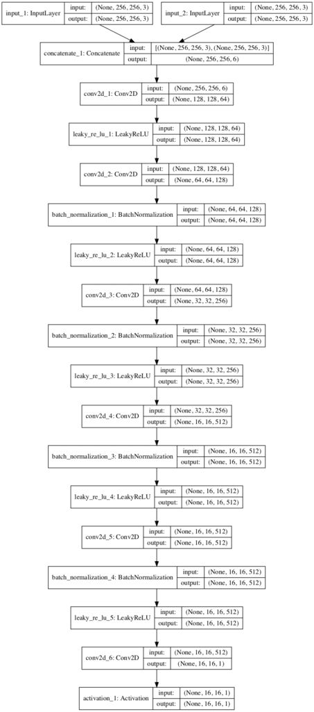
Plot of the PatchGAN Model Used in the Pix2Pix GAN Architecture
Now that we know how to implement the PatchGAN discriminator model, we can now look at implementing the U-Net generator model.
How to Implement the U-Net Generator Model
The generator model for the Pix2Pix GAN is implemented as a U-Net.
The U-Net model is an encoder-decoder model for image translation where skip connections are used to connect layers in the encoder with corresponding layers in the decoder that have the same sized feature maps.
The encoder part of the model is comprised of convolutional layers that use a 2×2 stride to downsample the input source image down to a bottleneck layer. The decoder part of the model reads the bottleneck output and uses transpose convolutional layers to upsample to the required output image size.
… the input is passed through a series of layers that progressively downsample, until a bottleneck layer, at which point the process is reversed.
— Image-to-Image Translation with Conditional Adversarial Networks, 2016.
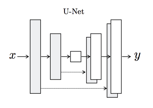
Architecture of the U-Net Generator Model
Taken from Image-to-Image Translation With Conditional Adversarial Networks.
Skip connections are added between the layers with the same sized feature maps so that the first downsampling layer is connected with the last upsampling layer, the second downsampling layer is connected with the second last upsampling layer, and so on. The connections concatenate the channels of the feature map in the downsampling layer with the feature map in the upsampling layer.
Specifically, we add skip connections between each layer i and layer n − i, where n is the total number of layers. Each skip connection simply concatenates all channels at layer i with those at layer n − i.
— Image-to-Image Translation with Conditional Adversarial Networks, 2016.
Unlike traditional generator models in the GAN architecture, the U-Net generator does not take a point from the latent space as input. Instead, dropout layers are used as a source of randomness both during training and when the model is used to make a prediction, e.g. generate an image at inference time.
Similarly, batch normalization is used in the same way during training and inference, meaning that statistics are calculated for each batch and not fixed at the end of the training process. This is referred to as instance normalization, specifically when the batch size is set to 1 as it is with the Pix2Pix model.
At inference time, we run the generator net in exactly the same manner as during the training phase. This differs from the usual protocol in that we apply dropout at test time, and we apply batch normalization using the statistics of the test batch, rather than aggregated statistics of the training batch.
— Image-to-Image Translation with Conditional Adversarial Networks, 2016.
In Keras, layers like Dropout and BatchNormalization operate differently during training and in inference model. We can set the “training” argument when calling these layers to “True” to ensure that they always operate in training-model, even when used during inference.
For example, a Dropout layer that will drop out during inference as well as training can be added to the model as follows:
...
g = Dropout(0.5)(g, training=True)
As with the discriminator model, the configuration details of the generator model are defined in the appendix of the paper and can be confirmed when comparing against the defineG_unet() function in the official Torch implementation.
The encoder uses blocks of Convolution-BatchNorm-LeakyReLU like the discriminator model, whereas the decoder model uses blocks of Convolution-BatchNorm-Dropout-ReLU with a dropout rate of 50%. All convolutional layers use a filter size of 4×4 and a stride of 2×2.
Let Ck denote a Convolution-BatchNorm-ReLU layer with k filters. CDk denotes a Convolution-BatchNormDropout-ReLU layer with a dropout rate of 50%. All convolutions are 4× 4 spatial filters applied with stride 2.
— Image-to-Image Translation with Conditional Adversarial Networks, 2016.
The architecture of the U-Net model is defined using the shorthand notation as:
- Encoder: C64-C128-C256-C512-C512-C512-C512-C512
- Decoder: CD512-CD1024-CD1024-C1024-C1024-C512-C256-C128
The last layer of the encoder is the bottleneck layer, which does not use batch normalization, according to an amendment to the paper and confirmation in the code, and uses a ReLU activation instead of LeakyRelu.
… the activations of the bottleneck layer are zeroed by the batchnorm operation, effectively making the innermost layer skipped. This issue can be fixed by removing batchnorm from this layer, as has been done in the public code
— Image-to-Image Translation with Conditional Adversarial Networks, 2016.
The number of filters in the U-Net decoder is a little misleading as it is the number of filters for the layer after concatenation with the equivalent layer in the encoder. This may become more clear when we create a plot of the model.
The output of the model uses a single convolutional layer with three channels, and tanh activation function is used in the output layer, common to GAN generator models. Batch normalization is not used in the first layer of the decoder.
After the last layer in the decoder, a convolution is applied to map to the number of output channels (3 in general […]), followed by a Tanh function […] BatchNorm is not applied to the first C64 layer in the encoder. All ReLUs in the encoder are leaky, with slope 0.2, while ReLUs in the decoder are not leaky.
— Image-to-Image Translation with Conditional Adversarial Networks, 2016.
Tying this all together, we can define a function named define_generator() that defines the U-Net encoder-decoder generator model. Two helper functions are also provided for defining encoder blocks of layers and decoder blocks of layers.
The complete example of defining the model is listed below.
# example of defining a u-net encoder-decoder generator model
from keras.initializers import RandomNormal
from keras.models import Model
from keras.models import Input
from keras.layers import Conv2D
from keras.layers import Conv2DTranspose
from keras.layers import LeakyReLU
from keras.layers import Activation
from keras.layers import Concatenate
from keras.layers import Dropout
from keras.layers import BatchNormalization
from keras.layers import LeakyReLU
from keras.utils.vis_utils import plot_model

# define an encoder block
def define_encoder_block(layer_in, n_filters, batchnorm=True):
	# weight initialization
	init = RandomNormal(stddev=0.02)
	# add downsampling layer
	g = Conv2D(n_filters, (4,4), strides=(2,2), padding='same', kernel_initializer=init)(layer_in)
	# conditionally add batch normalization
	if batchnorm:
		g = BatchNormalization()(g, training=True)
	# leaky relu activation
	g = LeakyReLU(alpha=0.2)(g)
	return g

# define a decoder block
def decoder_block(layer_in, skip_in, n_filters, dropout=True):
	# weight initialization
	init = RandomNormal(stddev=0.02)
	# add upsampling layer
	g = Conv2DTranspose(n_filters, (4,4), strides=(2,2), padding='same', kernel_initializer=init)(layer_in)
	# add batch normalization
	g = BatchNormalization()(g, training=True)
	# conditionally add dropout
	if dropout:
		g = Dropout(0.5)(g, training=True)
	# merge with skip connection
	g = Concatenate()([g, skip_in])
	# relu activation
	g = Activation('relu')(g)
	return g

# define the standalone generator model
def define_generator(image_shape=(256,256,3)):
	# weight initialization
	init = RandomNormal(stddev=0.02)
	# image input
	in_image = Input(shape=image_shape)
	# encoder model: C64-C128-C256-C512-C512-C512-C512-C512
	e1 = define_encoder_block(in_image, 64, batchnorm=False)
	e2 = define_encoder_block(e1, 128)
	e3 = define_encoder_block(e2, 256)
	e4 = define_encoder_block(e3, 512)
	e5 = define_encoder_block(e4, 512)
	e6 = define_encoder_block(e5, 512)
	e7 = define_encoder_block(e6, 512)
	# bottleneck, no batch norm and relu
	b = Conv2D(512, (4,4), strides=(2,2), padding='same', kernel_initializer=init)(e7)
	b = Activation('relu')(b)
	# decoder model: CD512-CD1024-CD1024-C1024-C1024-C512-C256-C128
	d1 = decoder_block(b, e7, 512)
	d2 = decoder_block(d1, e6, 512)
	d3 = decoder_block(d2, e5, 512)
	d4 = decoder_block(d3, e4, 512, dropout=False)
	d5 = decoder_block(d4, e3, 256, dropout=False)
	d6 = decoder_block(d5, e2, 128, dropout=False)
	d7 = decoder_block(d6, e1, 64, dropout=False)
	# output
	g = Conv2DTranspose(3, (4,4), strides=(2,2), padding='same', kernel_initializer=init)(d7)
	out_image = Activation('tanh')(g)
	# define model
	model = Model(in_image, out_image)
	return model

# define image shape
image_shape = (256,256,3)
# create the model
model = define_generator(image_shape)
# summarize the model
model.summary()
# plot the model
plot_model(model, to_file='generator_model_plot.png', show_shapes=True, show_layer_names=True)
Running the example first summarizes the model.
The model has a single input and output, but the skip connections make the summary difficult to read.
__________________________________________________________________________________________________
Layer (type)                    Output Shape         Param #     Connected to
==================================================================================================
input_1 (InputLayer)            (None, 256, 256, 3)  0
__________________________________________________________________________________________________
conv2d_1 (Conv2D)               (None, 128, 128, 64) 3136        input_1[0][0]
__________________________________________________________________________________________________
leaky_re_lu_1 (LeakyReLU)       (None, 128, 128, 64) 0           conv2d_1[0][0]
__________________________________________________________________________________________________
conv2d_2 (Conv2D)               (None, 64, 64, 128)  131200      leaky_re_lu_1[0][0]
__________________________________________________________________________________________________
batch_normalization_1 (BatchNor (None, 64, 64, 128)  512         conv2d_2[0][0]
__________________________________________________________________________________________________
leaky_re_lu_2 (LeakyReLU)       (None, 64, 64, 128)  0           batch_normalization_1[0][0]
__________________________________________________________________________________________________
conv2d_3 (Conv2D)               (None, 32, 32, 256)  524544      leaky_re_lu_2[0][0]
__________________________________________________________________________________________________
batch_normalization_2 (BatchNor (None, 32, 32, 256)  1024        conv2d_3[0][0]
__________________________________________________________________________________________________
leaky_re_lu_3 (LeakyReLU)       (None, 32, 32, 256)  0           batch_normalization_2[0][0]
__________________________________________________________________________________________________
conv2d_4 (Conv2D)               (None, 16, 16, 512)  2097664     leaky_re_lu_3[0][0]
__________________________________________________________________________________________________
batch_normalization_3 (BatchNor (None, 16, 16, 512)  2048        conv2d_4[0][0]
__________________________________________________________________________________________________
leaky_re_lu_4 (LeakyReLU)       (None, 16, 16, 512)  0           batch_normalization_3[0][0]
__________________________________________________________________________________________________
conv2d_5 (Conv2D)               (None, 8, 8, 512)    4194816     leaky_re_lu_4[0][0]
__________________________________________________________________________________________________
batch_normalization_4 (BatchNor (None, 8, 8, 512)    2048        conv2d_5[0][0]
__________________________________________________________________________________________________
leaky_re_lu_5 (LeakyReLU)       (None, 8, 8, 512)    0           batch_normalization_4[0][0]
__________________________________________________________________________________________________
conv2d_6 (Conv2D)               (None, 4, 4, 512)    4194816     leaky_re_lu_5[0][0]
__________________________________________________________________________________________________
batch_normalization_5 (BatchNor (None, 4, 4, 512)    2048        conv2d_6[0][0]
__________________________________________________________________________________________________
leaky_re_lu_6 (LeakyReLU)       (None, 4, 4, 512)    0           batch_normalization_5[0][0]
__________________________________________________________________________________________________
conv2d_7 (Conv2D)               (None, 2, 2, 512)    4194816     leaky_re_lu_6[0][0]
__________________________________________________________________________________________________
batch_normalization_6 (BatchNor (None, 2, 2, 512)    2048        conv2d_7[0][0]
__________________________________________________________________________________________________
leaky_re_lu_7 (LeakyReLU)       (None, 2, 2, 512)    0           batch_normalization_6[0][0]
__________________________________________________________________________________________________
conv2d_8 (Conv2D)               (None, 1, 1, 512)    4194816     leaky_re_lu_7[0][0]
__________________________________________________________________________________________________
activation_1 (Activation)       (None, 1, 1, 512)    0           conv2d_8[0][0]
__________________________________________________________________________________________________
conv2d_transpose_1 (Conv2DTrans (None, 2, 2, 512)    4194816     activation_1[0][0]
__________________________________________________________________________________________________
batch_normalization_7 (BatchNor (None, 2, 2, 512)    2048        conv2d_transpose_1[0][0]
__________________________________________________________________________________________________
dropout_1 (Dropout)             (None, 2, 2, 512)    0           batch_normalization_7[0][0]
__________________________________________________________________________________________________
concatenate_1 (Concatenate)     (None, 2, 2, 1024)   0           dropout_1[0][0]
                                                                 leaky_re_lu_7[0][0]
__________________________________________________________________________________________________
activation_2 (Activation)       (None, 2, 2, 1024)   0           concatenate_1[0][0]
__________________________________________________________________________________________________
conv2d_transpose_2 (Conv2DTrans (None, 4, 4, 512)    8389120     activation_2[0][0]
__________________________________________________________________________________________________
batch_normalization_8 (BatchNor (None, 4, 4, 512)    2048        conv2d_transpose_2[0][0]
__________________________________________________________________________________________________
dropout_2 (Dropout)             (None, 4, 4, 512)    0           batch_normalization_8[0][0]
__________________________________________________________________________________________________
concatenate_2 (Concatenate)     (None, 4, 4, 1024)   0           dropout_2[0][0]
                                                                 leaky_re_lu_6[0][0]
__________________________________________________________________________________________________
activation_3 (Activation)       (None, 4, 4, 1024)   0           concatenate_2[0][0]
__________________________________________________________________________________________________
conv2d_transpose_3 (Conv2DTrans (None, 8, 8, 512)    8389120     activation_3[0][0]
__________________________________________________________________________________________________
batch_normalization_9 (BatchNor (None, 8, 8, 512)    2048        conv2d_transpose_3[0][0]
__________________________________________________________________________________________________
dropout_3 (Dropout)             (None, 8, 8, 512)    0           batch_normalization_9[0][0]
__________________________________________________________________________________________________
concatenate_3 (Concatenate)     (None, 8, 8, 1024)   0           dropout_3[0][0]
                                                                 leaky_re_lu_5[0][0]
__________________________________________________________________________________________________
activation_4 (Activation)       (None, 8, 8, 1024)   0           concatenate_3[0][0]
__________________________________________________________________________________________________
conv2d_transpose_4 (Conv2DTrans (None, 16, 16, 512)  8389120     activation_4[0][0]
__________________________________________________________________________________________________
batch_normalization_10 (BatchNo (None, 16, 16, 512)  2048        conv2d_transpose_4[0][0]
__________________________________________________________________________________________________
concatenate_4 (Concatenate)     (None, 16, 16, 1024) 0           batch_normalization_10[0][0]
                                                                 leaky_re_lu_4[0][0]
__________________________________________________________________________________________________
activation_5 (Activation)       (None, 16, 16, 1024) 0           concatenate_4[0][0]
__________________________________________________________________________________________________
conv2d_transpose_5 (Conv2DTrans (None, 32, 32, 256)  4194560     activation_5[0][0]
__________________________________________________________________________________________________
batch_normalization_11 (BatchNo (None, 32, 32, 256)  1024        conv2d_transpose_5[0][0]
__________________________________________________________________________________________________
concatenate_5 (Concatenate)     (None, 32, 32, 512)  0           batch_normalization_11[0][0]
                                                                 leaky_re_lu_3[0][0]
__________________________________________________________________________________________________
activation_6 (Activation)       (None, 32, 32, 512)  0           concatenate_5[0][0]
__________________________________________________________________________________________________
conv2d_transpose_6 (Conv2DTrans (None, 64, 64, 128)  1048704     activation_6[0][0]
__________________________________________________________________________________________________
batch_normalization_12 (BatchNo (None, 64, 64, 128)  512         conv2d_transpose_6[0][0]
__________________________________________________________________________________________________
concatenate_6 (Concatenate)     (None, 64, 64, 256)  0           batch_normalization_12[0][0]
                                                                 leaky_re_lu_2[0][0]
__________________________________________________________________________________________________
activation_7 (Activation)       (None, 64, 64, 256)  0           concatenate_6[0][0]
__________________________________________________________________________________________________
conv2d_transpose_7 (Conv2DTrans (None, 128, 128, 64) 262208      activation_7[0][0]
__________________________________________________________________________________________________
batch_normalization_13 (BatchNo (None, 128, 128, 64) 256         conv2d_transpose_7[0][0]
__________________________________________________________________________________________________
concatenate_7 (Concatenate)     (None, 128, 128, 128 0           batch_normalization_13[0][0]
                                                                 leaky_re_lu_1[0][0]
__________________________________________________________________________________________________
activation_8 (Activation)       (None, 128, 128, 128 0           concatenate_7[0][0]
__________________________________________________________________________________________________
conv2d_transpose_8 (Conv2DTrans (None, 256, 256, 3)  6147        activation_8[0][0]
__________________________________________________________________________________________________
activation_9 (Activation)       (None, 256, 256, 3)  0           conv2d_transpose_8[0][0]
==================================================================================================
Total params: 54,429,315
Trainable params: 54,419,459
Non-trainable params: 9,856
__________________________________________________________________________________________________
A plot of the model is created showing much the same information in a graphical form. The model is complex, and the plot helps to understand the skip connections and their impact on the number of filters in the decoder.
Note: creating the plot assumes that pydot and pygraphviz libraries are installed. If this is a problem, you can comment out the import and call to the plot_model() function.
Working backward from the output layer, if we look at the Concatenate layers and the first Conv2DTranspose layer of the decoder, we can see the number of channels as:
- [128, 256, 512, 1024, 1024, 1024, 1024, 512].
Reversing this list gives the stated configuration of the number of filters for each layer in the decoder from the paper of:
- CD512-CD1024-CD1024-C1024-C1024-C512-C256-C128
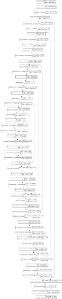
Plot of the U-Net Encoder-Decoder Model Used in the Pix2Pix GAN Architecture
Now that we have defined both models, we can look at how the generator model is updated via the discriminator model.
How to Implement Adversarial and L1 Loss
The discriminator model can be updated directly, whereas the generator model must be updated via the discriminator model.
This can be achieved by defining a new composite model in Keras that connects the output of the generator model as input to the discriminator model. The discriminator model can then predict whether a generated image is real or fake. We can update the weights of the composite model in such a way that the generated image has the label of “real” instead of “fake“, which will cause the generator weights to be updated towards generating a better fake image. We can also mark the discriminator weights as not trainable in this context, to avoid the misleading update.
Additionally, the generator needs to be updated to better match the targeted translation of the input image. This means that the composite model must also output the generated image directly, allowing it to be compared to the target image.
Therefore, we can summarize the inputs and outputs of this composite model as follows:
- Inputs: Source image
- Outputs: Classification of real/fake, generated target image.
The weights of the generator will be updated via both adversarial loss via the discriminator output and L1 loss via the direct image output. The loss scores are added together, where the L1 loss is treated as a regularizing term and weighted via a hyperparameter called lambda, set to 100.
- loss = adversarial loss + lambda * L1 loss
The define_gan() function below implements this, taking the defined generator and discriminator models as input and creating the composite GAN model that can be used to update the generator model weights.
The source image input is provided both to the generator and the discriminator as input and the output of the generator is also connected to the discriminator as input.
Two loss functions are specified when the model is compiled for the discriminator and generator outputs respectively. The loss_weights argument is used to define the weighting of each loss when added together to update the generator model weights.
# define the combined generator and discriminator model, for updating the generator
def define_gan(g_model, d_model, image_shape):
	# make weights in the discriminator not trainable
	d_model.trainable = False
	# define the source image
	in_src = Input(shape=image_shape)
	# connect the source image to the generator input
	gen_out = g_model(in_src)
	# connect the source input and generator output to the discriminator input
	dis_out = d_model([in_src, gen_out])
	# src image as input, generated image and classification output
	model = Model(in_src, [dis_out, gen_out])
	# compile model
	opt = Adam(lr=0.0002, beta_1=0.5)
	model.compile(loss=['binary_crossentropy', 'mae'], optimizer=opt, loss_weights=[1,100])
	return model
Tying this together with the model definitions from the previous sections, the complete example is listed below.
# example of defining a composite model for training the generator model
from keras.optimizers import Adam
from keras.initializers import RandomNormal
from keras.models import Model
from keras.models import Input
from keras.layers import Conv2D
from keras.layers import Conv2DTranspose
from keras.layers import LeakyReLU
from keras.layers import Activation
from keras.layers import Concatenate
from keras.layers import Dropout
from keras.layers import BatchNormalization
from keras.layers import LeakyReLU
from keras.utils.vis_utils import plot_model

# define the discriminator model
def define_discriminator(image_shape):
	# weight initialization
	init = RandomNormal(stddev=0.02)
	# source image input
	in_src_image = Input(shape=image_shape)
	# target image input
	in_target_image = Input(shape=image_shape)
	# concatenate images channel-wise
	merged = Concatenate()([in_src_image, in_target_image])
	# C64
	d = Conv2D(64, (4,4), strides=(2,2), padding='same', kernel_initializer=init)(merged)
	d = LeakyReLU(alpha=0.2)(d)
	# C128
	d = Conv2D(128, (4,4), strides=(2,2), padding='same', kernel_initializer=init)(d)
	d = BatchNormalization()(d)
	d = LeakyReLU(alpha=0.2)(d)
	# C256
	d = Conv2D(256, (4,4), strides=(2,2), padding='same', kernel_initializer=init)(d)
	d = BatchNormalization()(d)
	d = LeakyReLU(alpha=0.2)(d)
	# C512
	d = Conv2D(512, (4,4), strides=(2,2), padding='same', kernel_initializer=init)(d)
	d = BatchNormalization()(d)
	d = LeakyReLU(alpha=0.2)(d)
	# second last output layer
	d = Conv2D(512, (4,4), padding='same', kernel_initializer=init)(d)
	d = BatchNormalization()(d)
	d = LeakyReLU(alpha=0.2)(d)
	# patch output
	d = Conv2D(1, (4,4), padding='same', kernel_initializer=init)(d)
	patch_out = Activation('sigmoid')(d)
	# define model
	model = Model([in_src_image, in_target_image], patch_out)
	# compile model
	opt = Adam(lr=0.0002, beta_1=0.5)
	model.compile(loss='binary_crossentropy', optimizer=opt, loss_weights=[0.5])
	return model

# define an encoder block
def define_encoder_block(layer_in, n_filters, batchnorm=True):
	# weight initialization
	init = RandomNormal(stddev=0.02)
	# add downsampling layer
	g = Conv2D(n_filters, (4,4), strides=(2,2), padding='same', kernel_initializer=init)(layer_in)
	# conditionally add batch normalization
	if batchnorm:
		g = BatchNormalization()(g, training=True)
	# leaky relu activation
	g = LeakyReLU(alpha=0.2)(g)
	return g

# define a decoder block
def decoder_block(layer_in, skip_in, n_filters, dropout=True):
	# weight initialization
	init = RandomNormal(stddev=0.02)
	# add upsampling layer
	g = Conv2DTranspose(n_filters, (4,4), strides=(2,2), padding='same', kernel_initializer=init)(layer_in)
	# add batch normalization
	g = BatchNormalization()(g, training=True)
	# conditionally add dropout
	if dropout:
		g = Dropout(0.5)(g, training=True)
	# merge with skip connection
	g = Concatenate()([g, skip_in])
	# relu activation
	g = Activation('relu')(g)
	return g

# define the standalone generator model
def define_generator(image_shape=(256,256,3)):
	# weight initialization
	init = RandomNormal(stddev=0.02)
	# image input
	in_image = Input(shape=image_shape)
	# encoder model: C64-C128-C256-C512-C512-C512-C512-C512
	e1 = define_encoder_block(in_image, 64, batchnorm=False)
	e2 = define_encoder_block(e1, 128)
	e3 = define_encoder_block(e2, 256)
	e4 = define_encoder_block(e3, 512)
	e5 = define_encoder_block(e4, 512)
	e6 = define_encoder_block(e5, 512)
	e7 = define_encoder_block(e6, 512)
	# bottleneck, no batch norm and relu
	b = Conv2D(512, (4,4), strides=(2,2), padding='same', kernel_initializer=init)(e7)
	b = Activation('relu')(b)
	# decoder model: CD512-CD1024-CD1024-C1024-C1024-C512-C256-C128
	d1 = decoder_block(b, e7, 512)
	d2 = decoder_block(d1, e6, 512)
	d3 = decoder_block(d2, e5, 512)
	d4 = decoder_block(d3, e4, 512, dropout=False)
	d5 = decoder_block(d4, e3, 256, dropout=False)
	d6 = decoder_block(d5, e2, 128, dropout=False)
	d7 = decoder_block(d6, e1, 64, dropout=False)
	# output
	g = Conv2DTranspose(3, (4,4), strides=(2,2), padding='same', kernel_initializer=init)(d7)
	out_image = Activation('tanh')(g)
	# define model
	model = Model(in_image, out_image)
	return model

# define the combined generator and discriminator model, for updating the generator
def define_gan(g_model, d_model, image_shape):
	# make weights in the discriminator not trainable
	d_model.trainable = False
	# define the source image
	in_src = Input(shape=image_shape)
	# connect the source image to the generator input
	gen_out = g_model(in_src)
	# connect the source input and generator output to the discriminator input
	dis_out = d_model([in_src, gen_out])
	# src image as input, generated image and classification output
	model = Model(in_src, [dis_out, gen_out])
	# compile model
	opt = Adam(lr=0.0002, beta_1=0.5)
	model.compile(loss=['binary_crossentropy', 'mae'], optimizer=opt, loss_weights=[1,100])
	return model

# define image shape
image_shape = (256,256,3)
# define the models
d_model = define_discriminator(image_shape)
g_model = define_generator(image_shape)
# define the composite model
gan_model = define_gan(g_model, d_model, image_shape)
# summarize the model
gan_model.summary()
# plot the model
plot_model(gan_model, to_file='gan_model_plot.png', show_shapes=True, show_layer_names=True)
Running the example first summarizes the composite model, showing the 256×256 image input, the same shaped output from model_2 (the generator) and the PatchGAN classification prediction from model_1 (the discriminator).
__________________________________________________________________________________________________
Layer (type)                    Output Shape         Param #     Connected to
==================================================================================================
input_4 (InputLayer)            (None, 256, 256, 3)  0
__________________________________________________________________________________________________
model_2 (Model)                 (None, 256, 256, 3)  54429315    input_4[0][0]
__________________________________________________________________________________________________
model_1 (Model)                 (None, 16, 16, 1)    6968257     input_4[0][0]
                                                                 model_2[1][0]
==================================================================================================
Total params: 61,397,572
Trainable params: 54,419,459
Non-trainable params: 6,978,113
__________________________________________________________________________________________________
A plot of the composite model is also created, showing how the input image flows into the generator and discriminator, and that the model has two outputs or end-points from each of the two models.
Note: creating the plot assumes that pydot and pygraphviz libraries are installed. If this is a problem, you can comment out the import and call to the plot_model() function.
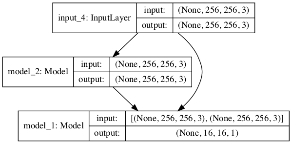
Plot of the Composite GAN Model Used to Train the Generator in the Pix2Pix GAN Architecture
How to Update Model Weights
Training the defined models is relatively straightforward.
First, we must define a helper function that will select a batch of real source and target images and the associated output (1.0). Here, the dataset is a list of two arrays of images.
# select a batch of random samples, returns images and target
def generate_real_samples(dataset, n_samples, patch_shape):
	# unpack dataset
	trainA, trainB = dataset
	# choose random instances
	ix = randint(0, trainA.shape[0], n_samples)
	# retrieve selected images
	X1, X2 = trainA[ix], trainB[ix]
	# generate 'real' class labels (1)
	y = ones((n_samples, patch_shape, patch_shape, 1))
	return [X1, X2], y
Similarly, we need a function to generate a batch of fake images and the associated output (0.0). Here, the samples are an array of source images for which target images will be generated.
# generate a batch of images, returns images and targets
def generate_fake_samples(g_model, samples, patch_shape):
	# generate fake instance
	X = g_model.predict(samples)
	# create 'fake' class labels (0)
	y = zeros((len(X), patch_shape, patch_shape, 1))
	return X, y
Now, we can define the steps of a single training iteration.
First, we must select a batch of source and target images by calling generate_real_samples().
Typically, the batch size (n_batch) is set to 1. In this case, we will assume 256×256 input images, which means the n_patch for the PatchGAN discriminator will be 16 to indicate a 16×16 output feature map.
...
# select a batch of real samples
[X_realA, X_realB], y_real = generate_real_samples(dataset, n_batch, n_patch)
Next, we can use the batches of selected real source images to generate corresponding batches of generated or fake target images.
...
# generate a batch of fake samples
X_fakeB, y_fake = generate_fake_samples(g_model, X_realA, n_patch)
We can then use the real and fake images, as well as their targets, to update the standalone discriminator model.
...
# update discriminator for real samples
d_loss1 = d_model.train_on_batch([X_realA, X_realB], y_real)
# update discriminator for generated samples
d_loss2 = d_model.train_on_batch([X_realA, X_fakeB], y_fake)
So far, this is normal for updating a GAN in Keras.
Next, we can update the generator model via adversarial loss and L1 loss. Recall that the composite GAN model takes a batch of source images as input and predicts first the classification of real/fake and second the generated target. Here, we provide a target to indicate the generated images are “real” (class=1) to the discriminator output of the composite model. The real target images are provided for calculating the L1 loss between them and the generated target images.
We have two loss functions, but three loss values calculated for a batch update, where only the first loss value is of interest as it is the weighted sum of the adversarial and L1 loss values for the batch.
...
# update the generator
g_loss, _, _ = gan_model.train_on_batch(X_realA, [y_real, X_realB])
That’s all there is to it.
We can define all of this in a function called train() that takes the defined models and a loaded dataset (as a list of two NumPy arrays) and trains the models.
# train pix2pix models
def train(d_model, g_model, gan_model, dataset, n_epochs=100, n_batch=1, n_patch=16):
	# unpack dataset
	trainA, trainB = dataset
	# calculate the number of batches per training epoch
	bat_per_epo = int(len(trainA) / n_batch)
	# calculate the number of training iterations
	n_steps = bat_per_epo * n_epochs
	# manually enumerate epochs
	for i in range(n_steps):
		# select a batch of real samples
		[X_realA, X_realB], y_real = generate_real_samples(dataset, n_batch, n_patch)
		# generate a batch of fake samples
		X_fakeB, y_fake = generate_fake_samples(g_model, X_realA, n_patch)
		# update discriminator for real samples
		d_loss1 = d_model.train_on_batch([X_realA, X_realB], y_real)
		# update discriminator for generated samples
		d_loss2 = d_model.train_on_batch([X_realA, X_fakeB], y_fake)
		# update the generator
		g_loss, _, _ = gan_model.train_on_batch(X_realA, [y_real, X_realB])
		# summarize performance
		print('>%d, d1[%.3f] d2[%.3f] g[%.3f]' % (i+1, d_loss1, d_loss2, g_loss))
The train function can then be called directly with our defined models and loaded dataset.
...
# load image data
dataset = ...
# train model
train(d_model, g_model, gan_model, dataset)
Further Reading
This section provides more resources on the topic if you are looking to go deeper.
Official
- Image-to-Image Translation with Conditional Adversarial Networks, 2016.
- Image-to-Image Translation with Conditional Adversarial Nets, Homepage.
- Image-to-image translation with conditional adversarial nets, GitHub.
- pytorch-CycleGAN-and-pix2pix, GitHub.
- Interactive Image-to-Image Demo, 2017.
- Pix2Pix Datasets
API
- Keras Datasets API.
- Keras Sequential Model API
- Keras Convolutional Layers API
- How can I “freeze” Keras layers?
Articles
- A guide to receptive field arithmetic for Convolutional Neural Networks, 2017.
- Question: PatchGAN Discriminator, 2017.
- receptive_field_sizes.m
Summary
In this tutorial, you discovered how to implement the Pix2Pix GAN architecture from scratch using the Keras deep learning framework.
Specifically, you learned:
- How to develop the PatchGAN discriminator model for the Pix2Pix GAN.
- How to develop the U-Net encoder-decoder generator model for the Pix2Pix GAN.
- How to implement the composite model for updating the generator and how to train both models.
Do you have any questions?
Ask your questions in the comments below and I will do my best to answer.
The post How to Implement Pix2Pix GAN Models From Scratch With Keras appeared first on Machine Learning Mastery.