
Author: Jason Brownlee
The Cycle Generative adversarial Network, or CycleGAN for short, is a generator model for converting images from one domain to another domain.
For example, the model can be used to translate images of horses to images of zebras, or photographs of city landscapes at night to city landscapes during the day.
The benefit of the CycleGAN model is that it can be trained without paired examples. That is, it does not require examples of photographs before and after the translation in order to train the model, e.g. photos of the same city landscape during the day and at night. Instead, it is able to use a collection of photographs from each domain and extract and harness the underlying style of images in the collection in order to perform the translation.
The model is very impressive but has an architecture that appears quite complicated to implement for beginners.
In this tutorial, you will discover how to implement the CycleGAN architecture from scratch using the Keras deep learning framework.
After completing this tutorial, you will know:
- How to implement the discriminator and generator models.
- How to define composite models to train the generator models via adversarial and cycle loss.
- How to implement the training process to update model weights each training iteration.
Discover how to develop DCGANs, conditional GANs, Pix2Pix, CycleGANs, and more with Keras in my new GANs book, with 29 step-by-step tutorials and full source code.
Let’s get started.

How to Develop CycleGAN Models From Scratch With Keras
Photo by anokarina, some rights reserved.
Tutorial Overview
This tutorial is divided into five parts; they are:
- What Is the CycleGAN Architecture?
- How to Implement the CycleGAN Discriminator Model
- How to Implement the CycleGAN Generator Model
- How to Implement Composite Models for Least Squares and Cycle Loss
- How to Update Discriminator and Generator Models
What Is the CycleGAN Architecture?
The CycleGAN model was described by Jun-Yan Zhu, et al. in their 2017 paper titled “Unpaired Image-to-Image Translation using Cycle-Consistent Adversarial Networks.”
The model architecture is comprised of two generator models: one generator (Generator-A) for generating images for the first domain (Domain-A) and the second generator (Generator-B) for generating images for the second domain (Domain-B).
- Generator-A -> Domain-A
- Generator-B -> Domain-B
The generator models perform image translation, meaning that the image generation process is conditional on an input image, specifically an image from the other domain. Generator-A takes an image from Domain-B as input and Generator-B takes an image from Domain-A as input.
- Domain-B -> Generator-A -> Domain-A
- Domain-A -> Generator-B -> Domain-B
Each generator has a corresponding discriminator model.
The first discriminator model (Discriminator-A) takes real images from Domain-A and generated images from Generator-A and predicts whether they are real or fake. The second discriminator model (Discriminator-B) takes real images from Domain-B and generated images from Generator-B and predicts whether they are real or fake.
- Domain-A -> Discriminator-A -> [Real/Fake]
- Domain-B -> Generator-A -> Discriminator-A -> [Real/Fake]
- Domain-B -> Discriminator-B -> [Real/Fake]
- Domain-A -> Generator-B -> Discriminator-B -> [Real/Fake]
The discriminator and generator models are trained in an adversarial zero-sum process, like normal GAN models.
The generators learn to better fool the discriminators and the discriminators learn to better detect fake images. Together, the models find an equilibrium during the training process.
Additionally, the generator models are regularized not just to create new images in the target domain, but instead create translated versions of the input images from the source domain. This is achieved by using generated images as input to the corresponding generator model and comparing the output image to the original images.
Passing an image through both generators is called a cycle. Together, each pair of generator models are trained to better reproduce the original source image, referred to as cycle consistency.
- Domain-B -> Generator-A -> Domain-A -> Generator-B -> Domain-B
- Domain-A -> Generator-B -> Domain-B -> Generator-A -> Domain-A
There is one further element to the architecture referred to as the identity mapping.
This is where a generator is provided with images as input from the target domain and is expected to generate the same image without change. This addition to the architecture is optional, although it results in a better matching of the color profile of the input image.
- Domain-A -> Generator-A -> Domain-A
- Domain-B -> Generator-B -> Domain-B
Now that we are familiar with the model architecture, we can take a closer look at each model in turn and how they can be implemented.
The paper provides a good description of the models and training process, although the official Torch implementation was used as the definitive description for each model and training process and provides the basis for the the model implementations described below.
Want to Develop GANs from Scratch?
Take my free 7-day email crash course now (with sample code).
Click to sign-up and also get a free PDF Ebook version of the course.
How to Implement the CycleGAN Discriminator Model
The discriminator model is responsible for taking a real or generated image as input and predicting whether it is real or fake.
The discriminator model is implemented as a PatchGAN model.
For the discriminator networks we use 70 × 70 PatchGANs, which aim to classify whether 70 × 70 overlapping image patches are real or fake.
— Unpaired Image-to-Image Translation using Cycle-Consistent Adversarial Networks, 2017.
The PatchGAN was described in the 2016 paper titled “Precomputed Real-time Texture Synthesis With Markovian Generative Adversarial Networks” and was used in the pix2pix model for image translation described in the 2016 paper titled “Image-to-Image Translation with Conditional Adversarial Networks.”
The architecture is described as discriminating an input image as real or fake by averaging the prediction for nxn squares or patches of the source image.
… we design a discriminator architecture – which we term a PatchGAN – that only penalizes structure at the scale of patches. This discriminator tries to classify if each NxN patch in an image is real or fake. We run this discriminator convolutionally across the image, averaging all responses to provide the ultimate output of D.
— Image-to-Image Translation with Conditional Adversarial Networks, 2016.
This can be implemented directly by using a somewhat standard deep convolutional discriminator model.
Instead of outputting a single value like a traditional discriminator model, the PatchGAN discriminator model can output a square or one-channel feature map of predictions. The 70×70 refers to the effective receptive field of the model on the input, not the actual shape of the output feature map.
The receptive field of a convolutional layer refers to the number of pixels that one output of the layer maps to in the input to the layer. The effective receptive field refers to the mapping of one pixel in the output of a deep convolutional model (multiple layers) to the input image. Here, the PatchGAN is an approach to designing a deep convolutional network based on the effective receptive field, where one output activation of the model maps to a 70×70 patch of the input image, regardless of the size of the input image.
The PatchGAN has the effect of predicting whether each 70×70 patch in the input image is real or fake. These predictions can then be averaged to give the output of the model (if needed) or compared directly to a matrix (or a vector if flattened) of expected values (e.g. 0 or 1 values).
The discriminator model described in the paper takes 256×256 color images as input and defines an explicit architecture that is used on all of the test problems. The architecture uses blocks of Conv2D-InstanceNorm-LeakyReLU layers, with 4×4 filters and a 2×2 stride.
Let Ck denote a 4×4 Convolution-InstanceNorm-LeakyReLU layer with k filters and stride 2. After the last layer, we apply a convolution to produce a 1-dimensional output. We do not use InstanceNorm for the first C64 layer. We use leaky ReLUs with a slope of 0.2.
— Unpaired Image-to-Image Translation using Cycle-Consistent Adversarial Networks, 2017.
The architecture for the discriminator is as follows:
- C64-C128-C256-C512
This is referred to as a 3-layer PatchGAN in the CycleGAN and Pix2Pix nomenclature, as excluding the first hidden layer, the model has three hidden layers that could be scaled up or down to give different sized PatchGAN models.
Not listed in the paper, the model also has a final hidden layer C512 with a 1×1 stride, and an output layer C1, also with a 1×1 stride with a linear activation function. Given the model is mostly used with 256×256 sized images as input, the size of the output feature map of activations is 16×16. If 128×128 images were used as input, then the size of the output feature map of activations would be 8×8.
The model does not use batch normalization; instead, instance normalization is used.
Instance normalization was described in the 2016 paper titled “Instance Normalization: The Missing Ingredient for Fast Stylization.” It is a very simple type of normalization and involves standardizing (e.g. scaling to a standard Gaussian) the values on each feature map.
The intent is to remove image-specific contrast information from the image during image generation, resulting in better generated images.
The key idea is to replace batch normalization layers in the generator architecture with instance normalization layers, and to keep them at test time (as opposed to freeze and simplify them out as done for batch normalization). Intuitively, the normalization process allows to remove instance-specific contrast information from the content image, which simplifies generation. In practice, this results in vastly improved images.
— Instance Normalization: The Missing Ingredient for Fast Stylization, 2016.
Although designed for generator models, it can also prove effective in discriminator models.
An implementation of instance normalization is provided in the keras-contrib project that provides early access to community-supplied Keras features.
The keras-contrib library can be installed via pip as follows:
sudo pip install git+https://www.github.com/keras-team/keras-contrib.git
Or, if you are using an Anaconda virtual environment, such as on EC2:
git clone https://www.github.com/keras-team/keras-contrib.git
cd keras-contrib
sudo ~/anaconda3/envs/tensorflow_p36/bin/python setup.py install
The new InstanceNormalization layer can then be used as follows:
...
from keras_contrib.layers.normalization.instancenormalization import InstanceNormalization
# define layer
layer = InstanceNormalization(axis=-1)
...
The “axis” argument is set to -1 to ensure that features are normalized per feature map.
The network weights are initialized to Gaussian random numbers with a standard deviation of 0.02, as is described for DCGANs more generally.
Weights are initialized from a Gaussian distribution N (0, 0.02).
— Unpaired Image-to-Image Translation using Cycle-Consistent Adversarial Networks, 2017.
The discriminator model is updated using a least squares loss (L2), a so-called Least-Squared Generative Adversarial Network, or LSGAN.
… we replace the negative log likelihood objective by a least-squares loss. This loss is more stable during training and generates higher quality results.
— Unpaired Image-to-Image Translation using Cycle-Consistent Adversarial Networks, 2017.
This can be implemented using “mean squared error” between the target values of class=1 for real images and class=0 for fake images.
Additionally, the paper suggests dividing the loss for the discriminator by half during training, in an effort to slow down updates to the discriminator relative to the generator.
In practice, we divide the objective by 2 while optimizing D, which slows down the rate at which D learns, relative to the rate of G.
— Unpaired Image-to-Image Translation using Cycle-Consistent Adversarial Networks, 2017.
This can be achieved by setting the “loss_weights” argument to 0.5 when compiling the model. Note that this weighting does not appear to be implemented in the official Torch implementation when updating discriminator models are defined in the fDx_basic() function.
We can tie all of this together in the example below with a define_discriminator() function that defines the PatchGAN discriminator. The model configuration matches the description in the appendix of the paper with additional details from the official Torch implementation defined in the defineD_n_layers() function.
# example of defining a 70x70 patchgan discriminator model
from keras.optimizers import Adam
from keras.initializers import RandomNormal
from keras.models import Model
from keras.models import Input
from keras.layers import Conv2D
from keras.layers import LeakyReLU
from keras.layers import Activation
from keras.layers import Concatenate
from keras.layers import BatchNormalization
from keras_contrib.layers.normalization.instancenormalization import InstanceNormalization
from keras.utils.vis_utils import plot_model

# define the discriminator model
def define_discriminator(image_shape):
	# weight initialization
	init = RandomNormal(stddev=0.02)
	# source image input
	in_image = Input(shape=image_shape)
	# C64
	d = Conv2D(64, (4,4), strides=(2,2), padding='same', kernel_initializer=init)(in_image)
	d = LeakyReLU(alpha=0.2)(d)
	# C128
	d = Conv2D(128, (4,4), strides=(2,2), padding='same', kernel_initializer=init)(d)
	d = InstanceNormalization(axis=-1)(d)
	d = LeakyReLU(alpha=0.2)(d)
	# C256
	d = Conv2D(256, (4,4), strides=(2,2), padding='same', kernel_initializer=init)(d)
	d = InstanceNormalization(axis=-1)(d)
	d = LeakyReLU(alpha=0.2)(d)
	# C512
	d = Conv2D(512, (4,4), strides=(2,2), padding='same', kernel_initializer=init)(d)
	d = InstanceNormalization(axis=-1)(d)
	d = LeakyReLU(alpha=0.2)(d)
	# second last output layer
	d = Conv2D(512, (4,4), padding='same', kernel_initializer=init)(d)
	d = InstanceNormalization(axis=-1)(d)
	d = LeakyReLU(alpha=0.2)(d)
	# patch output
	patch_out = Conv2D(1, (4,4), padding='same', kernel_initializer=init)(d)
	# define model
	model = Model(in_image, patch_out)
	# compile model
	model.compile(loss='mse', optimizer=Adam(lr=0.0002, beta_1=0.5), loss_weights=[0.5])
	return model

# define image shape
image_shape = (256,256,3)
# create the model
model = define_discriminator(image_shape)
# summarize the model
model.summary()
# plot the model
plot_model(model, to_file='discriminator_model_plot.png', show_shapes=True, show_layer_names=True)
Note: the plot_model() function requires that both the pydot and pygraphviz libraries are installed. If this is a problem, you can comment out both the import and call to this function.
Running the example summarizes the model showing the size inputs and outputs for each layer.
_________________________________________________________________
Layer (type)                 Output Shape              Param #
=================================================================
input_1 (InputLayer)         (None, 256, 256, 3)       0
_________________________________________________________________
conv2d_1 (Conv2D)            (None, 128, 128, 64)      3136
_________________________________________________________________
leaky_re_lu_1 (LeakyReLU)    (None, 128, 128, 64)      0
_________________________________________________________________
conv2d_2 (Conv2D)            (None, 64, 64, 128)       131200
_________________________________________________________________
instance_normalization_1 (In (None, 64, 64, 128)       256
_________________________________________________________________
leaky_re_lu_2 (LeakyReLU)    (None, 64, 64, 128)       0
_________________________________________________________________
conv2d_3 (Conv2D)            (None, 32, 32, 256)       524544
_________________________________________________________________
instance_normalization_2 (In (None, 32, 32, 256)       512
_________________________________________________________________
leaky_re_lu_3 (LeakyReLU)    (None, 32, 32, 256)       0
_________________________________________________________________
conv2d_4 (Conv2D)            (None, 16, 16, 512)       2097664
_________________________________________________________________
instance_normalization_3 (In (None, 16, 16, 512)       1024
_________________________________________________________________
leaky_re_lu_4 (LeakyReLU)    (None, 16, 16, 512)       0
_________________________________________________________________
conv2d_5 (Conv2D)            (None, 16, 16, 512)       4194816
_________________________________________________________________
instance_normalization_4 (In (None, 16, 16, 512)       1024
_________________________________________________________________
leaky_re_lu_5 (LeakyReLU)    (None, 16, 16, 512)       0
_________________________________________________________________
conv2d_6 (Conv2D)            (None, 16, 16, 1)         8193
=================================================================
Total params: 6,962,369
Trainable params: 6,962,369
Non-trainable params: 0
_________________________________________________________________
A plot of the model architecture is also created to help get an idea of the inputs, outputs, and transitions of the image data through the model.
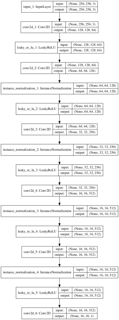
Plot of the PatchGAN Discriminator Model for the CycleGAN
How to Implement the CycleGAN Generator Model
The CycleGAN Generator model takes an image as input and generates a translated image as output.
The model uses a sequence of downsampling convolutional blocks to encode the input image, a number of residual network (ResNet) convolutional blocks to transform the image, and a number of upsampling convolutional blocks to generate the output image.
Let c7s1-k denote a 7×7 Convolution-InstanceNormReLU layer with k filters and stride 1. dk denotes a 3×3 Convolution-InstanceNorm-ReLU layer with k filters and stride 2. Reflection padding was used to reduce artifacts. Rk denotes a residual block that contains two 3 × 3 convolutional layers with the same number of filters on both layer. uk denotes a 3 × 3 fractional-strided-ConvolutionInstanceNorm-ReLU layer with k filters and stride 1/2.
— Unpaired Image-to-Image Translation using Cycle-Consistent Adversarial Networks, 2017.
The architecture for the 6-resnet block generator for 128×128 images is as follows:
- c7s1-64,d128,d256,R256,R256,R256,R256,R256,R256,u128,u64,c7s1-3
First, we need a function to define the ResNet blocks. These are blocks comprised of two 3×3 CNN layers where the input to the block is concatenated to the output of the block, channel-wise.
This is implemented in the resnet_block() function that creates two Conv-InstanceNorm blocks with 3×3 filters and 1×1 stride and without a ReLU activation after the second block, matching the official Torch implementation in the build_conv_block() function. Same padding is used instead of reflection padded recommended in the paper for simplicity.
# generator a resnet block
def resnet_block(n_filters, input_layer):
	# weight initialization
	init = RandomNormal(stddev=0.02)
	# first layer convolutional layer
	g = Conv2D(n_filters, (3,3), padding='same', kernel_initializer=init)(input_layer)
	g = InstanceNormalization(axis=-1)(g)
	g = Activation('relu')(g)
	# second convolutional layer
	g = Conv2D(n_filters, (3,3), padding='same', kernel_initializer=init)(g)
	g = InstanceNormalization(axis=-1)(g)
	# concatenate merge channel-wise with input layer
	g = Concatenate()([g, input_layer])
	return g
Next, we can define a function that will create the 9-resnet block version for 256×256 input images. This can easily be changed to the 6-resnet block version by setting image_shape to (128x128x3) and n_resnet function argument to 6.
Importantly, the model outputs pixel values with the shape as the input and pixel values are in the range [-1, 1], typical for GAN generator models.
# define the standalone generator model
def define_generator(image_shape=(256,256,3), n_resnet=9):
	# weight initialization
	init = RandomNormal(stddev=0.02)
	# image input
	in_image = Input(shape=image_shape)
	# c7s1-64
	g = Conv2D(64, (7,7), padding='same', kernel_initializer=init)(in_image)
	g = InstanceNormalization(axis=-1)(g)
	g = Activation('relu')(g)
	# d128
	g = Conv2D(128, (3,3), strides=(2,2), padding='same', kernel_initializer=init)(g)
	g = InstanceNormalization(axis=-1)(g)
	g = Activation('relu')(g)
	# d256
	g = Conv2D(256, (3,3), strides=(2,2), padding='same', kernel_initializer=init)(g)
	g = InstanceNormalization(axis=-1)(g)
	g = Activation('relu')(g)
	# R256
	for _ in range(n_resnet):
		g = resnet_block(256, g)
	# u128
	g = Conv2DTranspose(128, (3,3), strides=(2,2), padding='same', kernel_initializer=init)(g)
	g = InstanceNormalization(axis=-1)(g)
	g = Activation('relu')(g)
	# u64
	g = Conv2DTranspose(64, (3,3), strides=(2,2), padding='same', kernel_initializer=init)(g)
	g = InstanceNormalization(axis=-1)(g)
	g = Activation('relu')(g)
	# c7s1-3
	g = Conv2D(3, (7,7), padding='same', kernel_initializer=init)(g)
	g = InstanceNormalization(axis=-1)(g)
	out_image = Activation('tanh')(g)
	# define model
	model = Model(in_image, out_image)
	return model
The generator model is not compiled as it is trained via a composite model, seen in the next section.
Tying this together, the complete example is listed below.
# example of an encoder-decoder generator for the cyclegan
from keras.optimizers import Adam
from keras.models import Model
from keras.models import Input
from keras.layers import Conv2D
from keras.layers import Conv2DTranspose
from keras.layers import Activation
from keras.initializers import RandomNormal
from keras.layers import Concatenate
from keras_contrib.layers.normalization.instancenormalization import InstanceNormalization
from keras.utils.vis_utils import plot_model

# generator a resnet block
def resnet_block(n_filters, input_layer):
	# weight initialization
	init = RandomNormal(stddev=0.02)
	# first layer convolutional layer
	g = Conv2D(n_filters, (3,3), padding='same', kernel_initializer=init)(input_layer)
	g = InstanceNormalization(axis=-1)(g)
	g = Activation('relu')(g)
	# second convolutional layer
	g = Conv2D(n_filters, (3,3), padding='same', kernel_initializer=init)(g)
	g = InstanceNormalization(axis=-1)(g)
	# concatenate merge channel-wise with input layer
	g = Concatenate()([g, input_layer])
	return g

# define the standalone generator model
def define_generator(image_shape=(256,256,3), n_resnet=9):
	# weight initialization
	init = RandomNormal(stddev=0.02)
	# image input
	in_image = Input(shape=image_shape)
	# c7s1-64
	g = Conv2D(64, (7,7), padding='same', kernel_initializer=init)(in_image)
	g = InstanceNormalization(axis=-1)(g)
	g = Activation('relu')(g)
	# d128
	g = Conv2D(128, (3,3), strides=(2,2), padding='same', kernel_initializer=init)(g)
	g = InstanceNormalization(axis=-1)(g)
	g = Activation('relu')(g)
	# d256
	g = Conv2D(256, (3,3), strides=(2,2), padding='same', kernel_initializer=init)(g)
	g = InstanceNormalization(axis=-1)(g)
	g = Activation('relu')(g)
	# R256
	for _ in range(n_resnet):
		g = resnet_block(256, g)
	# u128
	g = Conv2DTranspose(128, (3,3), strides=(2,2), padding='same', kernel_initializer=init)(g)
	g = InstanceNormalization(axis=-1)(g)
	g = Activation('relu')(g)
	# u64
	g = Conv2DTranspose(64, (3,3), strides=(2,2), padding='same', kernel_initializer=init)(g)
	g = InstanceNormalization(axis=-1)(g)
	g = Activation('relu')(g)
	# c7s1-3
	g = Conv2D(3, (7,7), padding='same', kernel_initializer=init)(g)
	g = InstanceNormalization(axis=-1)(g)
	out_image = Activation('tanh')(g)
	# define model
	model = Model(in_image, out_image)
	return model

# create the model
model = define_generator()
# summarize the model
model.summary()
# plot the model
plot_model(model, to_file='generator_model_plot.png', show_shapes=True, show_layer_names=True)
Running the example first summarizes the model.
__________________________________________________________________________________________________
Layer (type)                    Output Shape         Param #     Connected to
==================================================================================================
input_1 (InputLayer)            (None, 256, 256, 3)  0
__________________________________________________________________________________________________
conv2d_1 (Conv2D)               (None, 256, 256, 64) 9472        input_1[0][0]
__________________________________________________________________________________________________
instance_normalization_1 (Insta (None, 256, 256, 64) 128         conv2d_1[0][0]
__________________________________________________________________________________________________
activation_1 (Activation)       (None, 256, 256, 64) 0           instance_normalization_1[0][0]
__________________________________________________________________________________________________
conv2d_2 (Conv2D)               (None, 128, 128, 128 73856       activation_1[0][0]
__________________________________________________________________________________________________
instance_normalization_2 (Insta (None, 128, 128, 128 256         conv2d_2[0][0]
__________________________________________________________________________________________________
activation_2 (Activation)       (None, 128, 128, 128 0           instance_normalization_2[0][0]
__________________________________________________________________________________________________
conv2d_3 (Conv2D)               (None, 64, 64, 256)  295168      activation_2[0][0]
__________________________________________________________________________________________________
instance_normalization_3 (Insta (None, 64, 64, 256)  512         conv2d_3[0][0]
__________________________________________________________________________________________________
activation_3 (Activation)       (None, 64, 64, 256)  0           instance_normalization_3[0][0]
__________________________________________________________________________________________________
conv2d_4 (Conv2D)               (None, 64, 64, 256)  590080      activation_3[0][0]
__________________________________________________________________________________________________
instance_normalization_4 (Insta (None, 64, 64, 256)  512         conv2d_4[0][0]
__________________________________________________________________________________________________
activation_4 (Activation)       (None, 64, 64, 256)  0           instance_normalization_4[0][0]
__________________________________________________________________________________________________
conv2d_5 (Conv2D)               (None, 64, 64, 256)  590080      activation_4[0][0]
__________________________________________________________________________________________________
instance_normalization_5 (Insta (None, 64, 64, 256)  512         conv2d_5[0][0]
__________________________________________________________________________________________________
concatenate_1 (Concatenate)     (None, 64, 64, 512)  0           instance_normalization_5[0][0]
                                                                 activation_3[0][0]
__________________________________________________________________________________________________
conv2d_6 (Conv2D)               (None, 64, 64, 256)  1179904     concatenate_1[0][0]
__________________________________________________________________________________________________
instance_normalization_6 (Insta (None, 64, 64, 256)  512         conv2d_6[0][0]
__________________________________________________________________________________________________
activation_5 (Activation)       (None, 64, 64, 256)  0           instance_normalization_6[0][0]
__________________________________________________________________________________________________
conv2d_7 (Conv2D)               (None, 64, 64, 256)  590080      activation_5[0][0]
__________________________________________________________________________________________________
instance_normalization_7 (Insta (None, 64, 64, 256)  512         conv2d_7[0][0]
__________________________________________________________________________________________________
concatenate_2 (Concatenate)     (None, 64, 64, 768)  0           instance_normalization_7[0][0]
                                                                 concatenate_1[0][0]
__________________________________________________________________________________________________
conv2d_8 (Conv2D)               (None, 64, 64, 256)  1769728     concatenate_2[0][0]
__________________________________________________________________________________________________
instance_normalization_8 (Insta (None, 64, 64, 256)  512         conv2d_8[0][0]
__________________________________________________________________________________________________
activation_6 (Activation)       (None, 64, 64, 256)  0           instance_normalization_8[0][0]
__________________________________________________________________________________________________
conv2d_9 (Conv2D)               (None, 64, 64, 256)  590080      activation_6[0][0]
__________________________________________________________________________________________________
instance_normalization_9 (Insta (None, 64, 64, 256)  512         conv2d_9[0][0]
__________________________________________________________________________________________________
concatenate_3 (Concatenate)     (None, 64, 64, 1024) 0           instance_normalization_9[0][0]
                                                                 concatenate_2[0][0]
__________________________________________________________________________________________________
conv2d_10 (Conv2D)              (None, 64, 64, 256)  2359552     concatenate_3[0][0]
__________________________________________________________________________________________________
instance_normalization_10 (Inst (None, 64, 64, 256)  512         conv2d_10[0][0]
__________________________________________________________________________________________________
activation_7 (Activation)       (None, 64, 64, 256)  0           instance_normalization_10[0][0]
__________________________________________________________________________________________________
conv2d_11 (Conv2D)              (None, 64, 64, 256)  590080      activation_7[0][0]
__________________________________________________________________________________________________
instance_normalization_11 (Inst (None, 64, 64, 256)  512         conv2d_11[0][0]
__________________________________________________________________________________________________
concatenate_4 (Concatenate)     (None, 64, 64, 1280) 0           instance_normalization_11[0][0]
                                                                 concatenate_3[0][0]
__________________________________________________________________________________________________
conv2d_12 (Conv2D)              (None, 64, 64, 256)  2949376     concatenate_4[0][0]
__________________________________________________________________________________________________
instance_normalization_12 (Inst (None, 64, 64, 256)  512         conv2d_12[0][0]
__________________________________________________________________________________________________
activation_8 (Activation)       (None, 64, 64, 256)  0           instance_normalization_12[0][0]
__________________________________________________________________________________________________
conv2d_13 (Conv2D)              (None, 64, 64, 256)  590080      activation_8[0][0]
__________________________________________________________________________________________________
instance_normalization_13 (Inst (None, 64, 64, 256)  512         conv2d_13[0][0]
__________________________________________________________________________________________________
concatenate_5 (Concatenate)     (None, 64, 64, 1536) 0           instance_normalization_13[0][0]
                                                                 concatenate_4[0][0]
__________________________________________________________________________________________________
conv2d_14 (Conv2D)              (None, 64, 64, 256)  3539200     concatenate_5[0][0]
__________________________________________________________________________________________________
instance_normalization_14 (Inst (None, 64, 64, 256)  512         conv2d_14[0][0]
__________________________________________________________________________________________________
activation_9 (Activation)       (None, 64, 64, 256)  0           instance_normalization_14[0][0]
__________________________________________________________________________________________________
conv2d_15 (Conv2D)              (None, 64, 64, 256)  590080      activation_9[0][0]
__________________________________________________________________________________________________
instance_normalization_15 (Inst (None, 64, 64, 256)  512         conv2d_15[0][0]
__________________________________________________________________________________________________
concatenate_6 (Concatenate)     (None, 64, 64, 1792) 0           instance_normalization_15[0][0]
                                                                 concatenate_5[0][0]
__________________________________________________________________________________________________
conv2d_16 (Conv2D)              (None, 64, 64, 256)  4129024     concatenate_6[0][0]
__________________________________________________________________________________________________
instance_normalization_16 (Inst (None, 64, 64, 256)  512         conv2d_16[0][0]
__________________________________________________________________________________________________
activation_10 (Activation)      (None, 64, 64, 256)  0           instance_normalization_16[0][0]
__________________________________________________________________________________________________
conv2d_17 (Conv2D)              (None, 64, 64, 256)  590080      activation_10[0][0]
__________________________________________________________________________________________________
instance_normalization_17 (Inst (None, 64, 64, 256)  512         conv2d_17[0][0]
__________________________________________________________________________________________________
concatenate_7 (Concatenate)     (None, 64, 64, 2048) 0           instance_normalization_17[0][0]
                                                                 concatenate_6[0][0]
__________________________________________________________________________________________________
conv2d_18 (Conv2D)              (None, 64, 64, 256)  4718848     concatenate_7[0][0]
__________________________________________________________________________________________________
instance_normalization_18 (Inst (None, 64, 64, 256)  512         conv2d_18[0][0]
__________________________________________________________________________________________________
activation_11 (Activation)      (None, 64, 64, 256)  0           instance_normalization_18[0][0]
__________________________________________________________________________________________________
conv2d_19 (Conv2D)              (None, 64, 64, 256)  590080      activation_11[0][0]
__________________________________________________________________________________________________
instance_normalization_19 (Inst (None, 64, 64, 256)  512         conv2d_19[0][0]
__________________________________________________________________________________________________
concatenate_8 (Concatenate)     (None, 64, 64, 2304) 0           instance_normalization_19[0][0]
                                                                 concatenate_7[0][0]
__________________________________________________________________________________________________
conv2d_20 (Conv2D)              (None, 64, 64, 256)  5308672     concatenate_8[0][0]
__________________________________________________________________________________________________
instance_normalization_20 (Inst (None, 64, 64, 256)  512         conv2d_20[0][0]
__________________________________________________________________________________________________
activation_12 (Activation)      (None, 64, 64, 256)  0           instance_normalization_20[0][0]
__________________________________________________________________________________________________
conv2d_21 (Conv2D)              (None, 64, 64, 256)  590080      activation_12[0][0]
__________________________________________________________________________________________________
instance_normalization_21 (Inst (None, 64, 64, 256)  512         conv2d_21[0][0]
__________________________________________________________________________________________________
concatenate_9 (Concatenate)     (None, 64, 64, 2560) 0           instance_normalization_21[0][0]
                                                                 concatenate_8[0][0]
__________________________________________________________________________________________________
conv2d_transpose_1 (Conv2DTrans (None, 128, 128, 128 2949248     concatenate_9[0][0]
__________________________________________________________________________________________________
instance_normalization_22 (Inst (None, 128, 128, 128 256         conv2d_transpose_1[0][0]
__________________________________________________________________________________________________
activation_13 (Activation)      (None, 128, 128, 128 0           instance_normalization_22[0][0]
__________________________________________________________________________________________________
conv2d_transpose_2 (Conv2DTrans (None, 256, 256, 64) 73792       activation_13[0][0]
__________________________________________________________________________________________________
instance_normalization_23 (Inst (None, 256, 256, 64) 128         conv2d_transpose_2[0][0]
__________________________________________________________________________________________________
activation_14 (Activation)      (None, 256, 256, 64) 0           instance_normalization_23[0][0]
__________________________________________________________________________________________________
conv2d_22 (Conv2D)              (None, 256, 256, 3)  9411        activation_14[0][0]
__________________________________________________________________________________________________
instance_normalization_24 (Inst (None, 256, 256, 3)  6           conv2d_22[0][0]
__________________________________________________________________________________________________
activation_15 (Activation)      (None, 256, 256, 3)  0           instance_normalization_24[0][0]
==================================================================================================
Total params: 35,276,553
Trainable params: 35,276,553
Non-trainable params: 0
__________________________________________________________________________________________________
A Plot of the generator model is also created, showing the skip connections in the ResNet blocks.
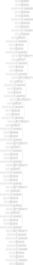
Plot of the Generator Model for the CycleGAN
How to Implement Composite Models for Least Squares and Cycle Loss
The generator models are not updated directly. Instead, the generator models are updated via composite models.
An update to each generator model involves changes to the model weights based on four concerns:
- Adversarial loss (L2 or mean squared error).
- Identity loss (L1 or mean absolute error).
- Forward cycle loss (L1 or mean absolute error).
- Backward cycle loss (L1 or mean absolute error).
The adversarial loss is the standard approach for updating the generator via the discriminator, although in this case, the least squares loss function is used instead of the negative log likelihood (e.g. binary cross entropy).
First, we can use our function to define the two generators and two discriminators used in the CycleGAN.
...
# input shape
image_shape = (256,256,3)
# generator: A -> B
g_model_AtoB = define_generator(image_shape)
# generator: B -> A
g_model_BtoA = define_generator(image_shape)
# discriminator: A -> [real/fake]
d_model_A = define_discriminator(image_shape)
# discriminator: B -> [real/fake]
d_model_B = define_discriminator(image_shape)
A composite model is required for each generator model that is responsible for only updating the weights of that generator model, although it is required to share the weights with the related discriminator model and the other generator model.
This can be achieved by marking the weights of the other models as not trainable in the context of the composite model to ensure we are only updating the intended generator.
...
# ensure the model we're updating is trainable
g_model_1.trainable = True
# mark discriminator as not trainable
d_model.trainable = False
# mark other generator model as not trainable
g_model_2.trainable = False
The model can be constructed piecewise using the Keras functional API.
The first step is to define the input of the real image from the source domain, pass it through our generator model, then connect the output of the generator to the discriminator and classify it as real or fake.
...
# discriminator element
input_gen = Input(shape=image_shape)
gen1_out = g_model_1(input_gen)
output_d = d_model(gen1_out)
Next, we can connect the identity mapping element with a new input for the real image from the target domain, pass it through our generator model, and output the (hopefully) untranslated image directly.
...
# identity element
input_id = Input(shape=image_shape)
output_id = g_model_1(input_id)
So far, we have a composite model with two real image inputs and a discriminator classification and identity image output. Next, we need to add the forward and backward cycles.
The forward cycle can be achieved by connecting the output of our generator to the other generator, the output of which can be compared to the input to our generator and should be identical.
...
# forward cycle
output_f = g_model_2(gen1_out)
The backward cycle is more complex and involves the input for the real image from the target domain passing through the other generator, then passing through our generator, which should match the real image from the target domain.
...
# backward cycle
gen2_out = g_model_2(input_id)
output_b = g_model_1(gen2_out)
That’s it.
We can then define this composite model with two inputs: one real image for the source and the target domain, and four outputs, one for the discriminator, one for the generator for the identity mapping, one for the other generator for the forward cycle, and one from our generator for the backward cycle.
...
# define model graph
model = Model([input_gen, input_id], [output_d, output_id, output_f, output_b])
The adversarial loss for the discriminator output uses least squares loss which is implemented as L2 or mean squared error. The outputs from the generators are compared to images and are optimized using L1 loss implemented as mean absolute error.
The generator is updated as a weighted average of the four loss values. The adversarial loss is weighted normally, whereas the forward and backward cycle loss is weighted using a parameter called lambda and is set to 10, e.g. 10 times more important than adversarial loss. The identity loss is also weighted as a fraction of the lambda parameter and is set to 0.5 * 10 or 5 in the official Torch implementation.
...
# compile model with weighting of least squares loss and L1 loss
model.compile(loss=['mse', 'mae', 'mae', 'mae'], loss_weights=[1, 5, 10, 10], optimizer=opt)
We can tie all of this together and define the function define_composite_model() for creating a composite model for training a given generator model.
# define a composite model for updating generators by adversarial and cycle loss
def define_composite_model(g_model_1, d_model, g_model_2, image_shape):
	# ensure the model we're updating is trainable
	g_model_1.trainable = True
	# mark discriminator as not trainable
	d_model.trainable = False
	# mark other generator model as not trainable
	g_model_2.trainable = False
	# discriminator element
	input_gen = Input(shape=image_shape)
	gen1_out = g_model_1(input_gen)
	output_d = d_model(gen1_out)
	# identity element
	input_id = Input(shape=image_shape)
	output_id = g_model_1(input_id)
	# forward cycle
	output_f = g_model_2(gen1_out)
	# backward cycle
	gen2_out = g_model_2(input_id)
	output_b = g_model_1(gen2_out)
	# define model graph
	model = Model([input_gen, input_id], [output_d, output_id, output_f, output_b])
	# define optimization algorithm configuration
	opt = Adam(lr=0.0002, beta_1=0.5)
	# compile model with weighting of least squares loss and L1 loss
	model.compile(loss=['mse', 'mae', 'mae', 'mae'], loss_weights=[1, 5, 10, 10], optimizer=opt)
	return model
This function can then be called to prepare a composite model for training both the g_model_AtoB generator model and the g_model_BtoA model; for example:
...
# composite: A -> B -> [real/fake, A]
c_model_AtoBtoA = define_composite_model(g_model_AtoB, d_model_B, g_model_BtoA, image_shape)
# composite: B -> A -> [real/fake, B]
c_model_BtoAtoB = define_composite_model(g_model_BtoA, d_model_A, g_model_AtoB, image_shape)
Summarizing and plotting the composite model is a bit of a mess as it does not help to see the inputs and outputs of the model clearly.
We can summarize the inputs and outputs for each of the composite models below. Recall that we are sharing or reusing the same set of weights if a given model is used more than once in the composite model.
Generator-A Composite Model
Only Generator-A weights are trainable and weights for other models and not trainable.
- Adversarial Loss: Domain-B -> Generator-A -> Domain-A -> Discriminator-A -> [real/fake]
- Identity Loss: Domain-A -> Generator-A -> Domain-A
- Forward Cycle Loss: Domain-B -> Generator-A -> Domain-A -> Generator-B -> Domain-B
- Backward Cycle Loss: Domain-A -> Generator-B -> Domain-B -> Generator-A -> Domain-A
Generator-B Composite Model
Only Generator-B weights are trainable and weights for other models are not trainable.
- Adversarial Loss: Domain-A -> Generator-B -> Domain-B -> Discriminator-B -> [real/fake]
- Identity Loss: Domain-B -> Generator-B -> Domain-B
- Forward Cycle Loss: Domain-A -> Generator-B -> Domain-B -> Generator-A -> Domain-A
- Backward Cycle Loss: Domain-B -> Generator-A -> Domain-A -> Generator-B -> Domain-B
A complete example of creating all of the models is listed below for completeness.
# example of defining composite models for training cyclegan generators
from keras.optimizers import Adam
from keras.models import Model
from keras.models import Sequential
from keras.models import Input
from keras.layers import Conv2D
from keras.layers import Conv2DTranspose
from keras.layers import Activation
from keras.layers import LeakyReLU
from keras.initializers import RandomNormal
from keras.layers import Concatenate
from keras_contrib.layers.normalization.instancenormalization import InstanceNormalization
from keras.utils.vis_utils import plot_model

# define the discriminator model
def define_discriminator(image_shape):
	# weight initialization
	init = RandomNormal(stddev=0.02)
	# source image input
	in_image = Input(shape=image_shape)
	# C64
	d = Conv2D(64, (4,4), strides=(2,2), padding='same', kernel_initializer=init)(in_image)
	d = LeakyReLU(alpha=0.2)(d)
	# C128
	d = Conv2D(128, (4,4), strides=(2,2), padding='same', kernel_initializer=init)(d)
	d = InstanceNormalization(axis=-1)(d)
	d = LeakyReLU(alpha=0.2)(d)
	# C256
	d = Conv2D(256, (4,4), strides=(2,2), padding='same', kernel_initializer=init)(d)
	d = InstanceNormalization(axis=-1)(d)
	d = LeakyReLU(alpha=0.2)(d)
	# C512
	d = Conv2D(512, (4,4), strides=(2,2), padding='same', kernel_initializer=init)(d)
	d = InstanceNormalization(axis=-1)(d)
	d = LeakyReLU(alpha=0.2)(d)
	# second last output layer
	d = Conv2D(512, (4,4), padding='same', kernel_initializer=init)(d)
	d = InstanceNormalization(axis=-1)(d)
	d = LeakyReLU(alpha=0.2)(d)
	# patch output
	patch_out = Conv2D(1, (4,4), padding='same', kernel_initializer=init)(d)
	# define model
	model = Model(in_image, patch_out)
	# compile model
	model.compile(loss='mse', optimizer=Adam(lr=0.0002, beta_1=0.5), loss_weights=[0.5])
	return model

# generator a resnet block
def resnet_block(n_filters, input_layer):
	# weight initialization
	init = RandomNormal(stddev=0.02)
	# first layer convolutional layer
	g = Conv2D(n_filters, (3,3), padding='same', kernel_initializer=init)(input_layer)
	g = InstanceNormalization(axis=-1)(g)
	g = Activation('relu')(g)
	# second convolutional layer
	g = Conv2D(n_filters, (3,3), padding='same', kernel_initializer=init)(g)
	g = InstanceNormalization(axis=-1)(g)
	# concatenate merge channel-wise with input layer
	g = Concatenate()([g, input_layer])
	return g

# define the standalone generator model
def define_generator(image_shape, n_resnet=9):
	# weight initialization
	init = RandomNormal(stddev=0.02)
	# image input
	in_image = Input(shape=image_shape)
	# c7s1-64
	g = Conv2D(64, (7,7), padding='same', kernel_initializer=init)(in_image)
	g = InstanceNormalization(axis=-1)(g)
	g = Activation('relu')(g)
	# d128
	g = Conv2D(128, (3,3), strides=(2,2), padding='same', kernel_initializer=init)(g)
	g = InstanceNormalization(axis=-1)(g)
	g = Activation('relu')(g)
	# d256
	g = Conv2D(256, (3,3), strides=(2,2), padding='same', kernel_initializer=init)(g)
	g = InstanceNormalization(axis=-1)(g)
	g = Activation('relu')(g)
	# R256
	for _ in range(n_resnet):
		g = resnet_block(256, g)
	# u128
	g = Conv2DTranspose(128, (3,3), strides=(2,2), padding='same', kernel_initializer=init)(g)
	g = InstanceNormalization(axis=-1)(g)
	g = Activation('relu')(g)
	# u64
	g = Conv2DTranspose(64, (3,3), strides=(2,2), padding='same', kernel_initializer=init)(g)
	g = InstanceNormalization(axis=-1)(g)
	g = Activation('relu')(g)
	# c7s1-3
	g = Conv2D(3, (7,7), padding='same', kernel_initializer=init)(g)
	g = InstanceNormalization(axis=-1)(g)
	out_image = Activation('tanh')(g)
	# define model
	model = Model(in_image, out_image)
	return model

# define a composite model for updating generators by adversarial and cycle loss
def define_composite_model(g_model_1, d_model, g_model_2, image_shape):
	# ensure the model we're updating is trainable
	g_model_1.trainable = True
	# mark discriminator as not trainable
	d_model.trainable = False
	# mark other generator model as not trainable
	g_model_2.trainable = False
	# discriminator element
	input_gen = Input(shape=image_shape)
	gen1_out = g_model_1(input_gen)
	output_d = d_model(gen1_out)
	# identity element
	input_id = Input(shape=image_shape)
	output_id = g_model_1(input_id)
	# forward cycle
	output_f = g_model_2(gen1_out)
	# backward cycle
	gen2_out = g_model_2(input_id)
	output_b = g_model_1(gen2_out)
	# define model graph
	model = Model([input_gen, input_id], [output_d, output_id, output_f, output_b])
	# define optimization algorithm configuration
	opt = Adam(lr=0.0002, beta_1=0.5)
	# compile model with weighting of least squares loss and L1 loss
	model.compile(loss=['mse', 'mae', 'mae', 'mae'], loss_weights=[1, 5, 10, 10], optimizer=opt)
	return model

# input shape
image_shape = (256,256,3)
# generator: A -> B
g_model_AtoB = define_generator(image_shape)
# generator: B -> A
g_model_BtoA = define_generator(image_shape)
# discriminator: A -> [real/fake]
d_model_A = define_discriminator(image_shape)
# discriminator: B -> [real/fake]
d_model_B = define_discriminator(image_shape)
# composite: A -> B -> [real/fake, A]
c_model_AtoB = define_composite_model(g_model_AtoB, d_model_B, g_model_BtoA, image_shape)
# composite: B -> A -> [real/fake, B]
c_model_BtoA = define_composite_model(g_model_BtoA, d_model_A, g_model_AtoB, image_shape)
How to Update Discriminator and Generator Models
Training the defined models is relatively straightforward.
First, we must define a helper function that will select a batch of real images and the associated target (1.0).
# select a batch of random samples, returns images and target
def generate_real_samples(dataset, n_samples, patch_shape):
	# choose random instances
	ix = randint(0, dataset.shape[0], n_samples)
	# retrieve selected images
	X = dataset[ix]
	# generate 'real' class labels (1)
	y = ones((n_samples, patch_shape, patch_shape, 1))
	return X, y
Similarly, we need a function to generate a batch of fake images and the associated target (0.0).
# generate a batch of images, returns images and targets
def generate_fake_samples(g_model, dataset, patch_shape):
	# generate fake instance
	X = g_model.predict(dataset)
	# create 'fake' class labels (0)
	y = zeros((len(X), patch_shape, patch_shape, 1))
	return X, y
Now, we can define the steps of a single training iteration. We will model the order of updates based on the implementation in the official Torch implementation in the OptimizeParameters() function (Note: the official code uses a more confusing inverted naming convention).
- Update Generator-B (A->B)
- Update Discriminator-B
- Update Generator-A (B->A)
- Update Discriminator-A
First, we must select a batch of real images by calling generate_real_samples() for both Domain-A and Domain-B.
Typically, the batch size (n_batch) is set to 1. In this case, we will assume 256×256 input images, which means the n_patch for the PatchGAN discriminator will be 16.
...
# select a batch of real samples
X_realA, y_realA = generate_real_samples(trainA, n_batch, n_patch)
X_realB, y_realB = generate_real_samples(trainB, n_batch, n_patch)
Next, we can use the batches of selected real images to generate corresponding batches of generated or fake images.
...
# generate a batch of fake samples
X_fakeA, y_fakeA = generate_fake_samples(g_model_BtoA, X_realB, n_patch)
X_fakeB, y_fakeB = generate_fake_samples(g_model_AtoB, X_realA, n_patch)
The paper describes using a pool of previously generated images from which examples are randomly selected and used to update the discriminator model, where the pool size was set to 50 images.
… [we] update the discriminators using a history of generated images rather than the ones produced by the latest generators. We keep an image buffer that stores the 50 previously created images.
— Unpaired Image-to-Image Translation using Cycle-Consistent Adversarial Networks, 2017.
This can be implemented using a list for each domain and a using a function to populate the pool, then randomly replace elements from the pool once it is at capacity.
The update_image_pool() function below implements this based on the official Torch implementation in image_pool.lua.
# update image pool for fake images
def update_image_pool(pool, images, max_size=50):
	selected = list()
	for image in images:
		if len(pool) < max_size:
			# stock the pool
			pool.append(image)
			selected.append(image)
		elif random() < 0.5:
			# use image, but don't add it to the pool
			selected.append(image)
		else:
			# replace an existing image and use replaced image
			ix = randint(0, len(pool))
			selected.append(pool[ix])
			pool[ix] = image
	return asarray(selected)
We can then update our image pool with generated fake images, the results of which can be used to train the discriminator models.
...
# update fakes from pool
X_fakeA = update_image_pool(poolA, X_fakeA)
X_fakeB = update_image_pool(poolB, X_fakeB)
Next, we can update Generator-A.
The train_on_batch() function will return a value for each of the four loss functions, one for each output, as well as the weighted sum (first value) used to update the model weights which we are interested in.
...
# update generator B->A via adversarial and cycle loss
g_loss2, _, _, _, _  = c_model_BtoA.train_on_batch([X_realB, X_realA], [y_realA, X_realA, X_realB, X_realA])
We can then update the discriminator model using the fake images that may or may not have come from the image pool.
...
# update discriminator for A -> [real/fake]
dA_loss1 = d_model_A.train_on_batch(X_realA, y_realA)
dA_loss2 = d_model_A.train_on_batch(X_fakeA, y_fakeA)
We can then do the same for the other generator and discriminator models.
...
# update generator A->B via adversarial and cycle loss
g_loss1, _, _, _, _ = c_model_AtoB.train_on_batch([X_realA, X_realB], [y_realB, X_realB, X_realA, X_realB])
# update discriminator for B -> [real/fake]
dB_loss1 = d_model_B.train_on_batch(X_realB, y_realB)
dB_loss2 = d_model_B.train_on_batch(X_fakeB, y_fakeB)
At the end of the training run, we can then report the current loss for the discriminator models on real and fake images and of each generator model.
...
# summarize performance
print('>%d, dA[%.3f,%.3f] dB[%.3f,%.3f] g[%.3f,%.3f]' % (i+1, dA_loss1,dA_loss2, dB_loss1,dB_loss2, g_loss1,g_loss2))
Tying this all together, we can define a function named train() that takes an instance of each of the defined models and a loaded dataset (list of two NumPy arrays, one for each domain) and trains the model.
A batch size of 1 is used as is described in the paper and the models are fit for 100 training epochs.
# train cyclegan models
def train(d_model_A, d_model_B, g_model_AtoB, g_model_BtoA, c_model_AtoB, c_model_BtoA, dataset):
	# define properties of the training run
	n_epochs, n_batch, = 100, 1
	# determine the output square shape of the discriminator
	n_patch = d_model_A.output_shape[1]
	# unpack dataset
	trainA, trainB = dataset
	# prepare image pool for fakes
	poolA, poolB = list(), list()
	# calculate the number of batches per training epoch
	bat_per_epo = int(len(trainA) / n_batch)
	# calculate the number of training iterations
	n_steps = bat_per_epo * n_epochs
	# manually enumerate epochs
	for i in range(n_steps):
		# select a batch of real samples
		X_realA, y_realA = generate_real_samples(trainA, n_batch, n_patch)
		X_realB, y_realB = generate_real_samples(trainB, n_batch, n_patch)
		# generate a batch of fake samples
		X_fakeA, y_fakeA = generate_fake_samples(g_model_BtoA, X_realB, n_patch)
		X_fakeB, y_fakeB = generate_fake_samples(g_model_AtoB, X_realA, n_patch)
		# update fakes from pool
		X_fakeA = update_image_pool(poolA, X_fakeA)
		X_fakeB = update_image_pool(poolB, X_fakeB)
		# update generator B->A via adversarial and cycle loss
		g_loss2, _, _, _, _  = c_model_BtoA.train_on_batch([X_realB, X_realA], [y_realA, X_realA, X_realB, X_realA])
		# update discriminator for A -> [real/fake]
		dA_loss1 = d_model_A.train_on_batch(X_realA, y_realA)
		dA_loss2 = d_model_A.train_on_batch(X_fakeA, y_fakeA)
		# update generator A->B via adversarial and cycle loss
		g_loss1, _, _, _, _ = c_model_AtoB.train_on_batch([X_realA, X_realB], [y_realB, X_realB, X_realA, X_realB])
		# update discriminator for B -> [real/fake]
		dB_loss1 = d_model_B.train_on_batch(X_realB, y_realB)
		dB_loss2 = d_model_B.train_on_batch(X_fakeB, y_fakeB)
		# summarize performance
		print('>%d, dA[%.3f,%.3f] dB[%.3f,%.3f] g[%.3f,%.3f]' % (i+1, dA_loss1,dA_loss2, dB_loss1,dB_loss2, g_loss1,g_loss2))
The train function can then be called directly with our defined models and loaded dataset.
...
# load a dataset as a list of two numpy arrays
dataset = ...
# train models
train(d_model_A, d_model_B, g_model_AtoB, g_model_BtoA, c_model_AtoB, c_model_BtoA, dataset)
As an improvement, it may be desirable to combine the update to each discriminator model into a single operation as is performed in the fDx_basic() function of the official implementation.
Additionally, the paper describes updating the models for another 100 epochs (200 in total), where the learning rate is decayed to 0.0. This too can be added as a minor extension to the training process.
Further Reading
This section provides more resources on the topic if you are looking to go deeper.
Papers
- Unpaired Image-to-Image Translation using Cycle-Consistent Adversarial Networks, 2017.
- Perceptual Losses for Real-Time Style Transfer and Super-Resolution, 2016.
- Image-to-Image Translation with Conditional Adversarial Networks, 2016.
- Least Squares Generative Adversarial Networks, 2016.
- Precomputed Real-time Texture Synthesis With Markovian Generative Adversarial Networks, 2016.
- Instance Normalization: The Missing Ingredient for Fast Stylization
- Layer Normalization
API
Projects
- CycleGAN Project (official), GitHub
- pytorch-CycleGAN-and-pix2pix (official), GitHub.
- CycleGAN Project Page (official)
- Keras-GAN: Keras implementations of Generative Adversarial Networks.
- CycleGAN-Keras: Keras implementation of CycleGAN using a tensorflow backend.
- cyclegan-keras: keras implementation of cycle-gan
Articles
Summary
In this tutorial, you discovered how to implement the CycleGAN architecture from scratch using the Keras deep learning framework.
Specifically, you learned:
- How to implement the discriminator and generator models.
- How to define composite models to train the generator models via adversarial and cycle loss.
- How to implement the training process to update model weights each training iteration.
Do you have any questions?
Ask your questions in the comments below and I will do my best to answer.
The post How to Implement CycleGAN Models From Scratch With Keras appeared first on Machine Learning Mastery.