
Author: Jason Brownlee
Cross-entropy is commonly used in machine learning as a loss function.
Cross-entropy is a measure from the field of information theory, building upon entropy and generally calculating the difference between two probability distributions. It is closely related to but is different from KL divergence that calculates the relative entropy between two probability distributions, whereas cross-entropy can be thought to calculate the total entropy between the distributions.
Cross-entropy is also related to and often confused with logistic loss, called log loss. Although the two measures are derived from a different source, when used as loss functions for classification models, both measures calculate the same quantity and can be used interchangeably.
In this tutorial, you will discover cross-entropy for machine learning.
After completing this tutorial, you will know:
- How to calculate cross-entropy from scratch and using standard machine learning libraries.
- Cross-entropy can be used as a loss function when optimizing classification models like logistic regression and artificial neural networks.
- Cross-entropy is different from KL divergence but can be calculated using KL divergence, and is different from log loss but calculates the same quantity when used as a loss function.
Discover bayes opimization, naive bayes, maximum likelihood, distributions, cross entropy, and much more in my new book, with 28 step-by-step tutorials and full Python source code.
Let’s get started.

A Gentle Introduction to Cross-Entropy for Machine Learning
Photo by Jerome Bon, some rights reserved.
Tutorial Overview
This tutorial is divided into five parts; they are:
- What Is Cross-Entropy?
- Difference Between Cross-Entropy and KL Divergence
- How to Calculate Cross-Entropy?
- Cross-Entropy as a Loss Function
- Difference Between Cross-Entropy and Log Loss
What Is Cross-Entropy?
Cross-entropy is a measure of the difference between two probability distributions for a given random variable or set of events.
Specifically, it builds upon the idea of entropy from information theory and calculates the average number of bits required to represent or transmit an event from one distribution compared to the other distribution.
… the cross entropy is the average number of bits needed to encode data coming from a source with distribution p when we use model q …
— Page 57, Machine Learning: A Probabilistic Perspective, 2012.
The intuition for this definition comes if we consider a target or underlying probability distribution P and an approximation of the target distribution Q, then the cross-entropy of Q from P is the number of additional bits to represent an event using Q instead of P.
The cross-entropy between two probability distributions, such as Q from P, can be stated formally as:
- H(P, Q)
Where H() is the cross-entropy function, P may be the target distribution and Q is the approximation of the target distribution.
Cross-entropy can be calculated using the probabilities of the events from P and Q, as follows:
- H(P, Q) = – sum x in X P(x) * log(Q(x))
Where P(x) is the probability of the event x in P, Q(x) is the probability of event x in Q and log is the base-2 logarithm, meaning that the results are in bits. If the base-e or natural logarithm is used instead, the result will have the units called nats.
This calculation is for discrete probability distributions, although a similar calculation can be used for continuous probability distributions using the integral across the events instead of the sum.
The result will be a positive number measured in bits and 0 if the two probability distributions are identical.
Note: this notation looks a lot like the joint probability, or more specifically, the joint entropy between P and Q. This is misleading as we are scoring the difference between probability distributions with cross-entropy. Whereas, joint entropy is a different concept that uses the same notation and instead calculates the uncertainty across two (or more) random variables.
Want to Learn Probability for Machine Learning
Take my free 7-day email crash course now (with sample code).
Click to sign-up and also get a free PDF Ebook version of the course.
Difference Between Cross-Entropy and KL Divergence
Cross-entropy is not KL Divergence.
Cross-entropy is related to divergence measures, such as the Kullback-Leibler, or KL, Divergence that quantifies how much one distribution differs from another.
Specifically, the KL divergence measures a very similar quantity to cross-entropy. It measures the average number of extra bits required to represent a message with Q instead of P, not the total number of bits.
In other words, the KL divergence is the average number of extra bits needed to encode the data, due to the fact that we used distribution q to encode the data instead of the true distribution p.
— Page 58, Machine Learning: A Probabilistic Perspective, 2012.
As such, the KL divergence is often referred to as the “relative entropy.”
- Cross-Entropy: Average number of total bits to represent an event from Q instead of P.
- Relative Entropy (KL Divergence): Average number of extra bits to represent an event from Q instead of P.
KL divergence can be calculated as the negative sum of probability of each event in P multiples by the log of the probability of the event in Q over the probability of the event in P. Typically, log base-2 so that the result is measured in bits.
- KL(P || Q) = – sum x in X P(x) * log(Q(x) / P(x))
The value within the sum is the divergence for a given event.
As such, we can calculate the cross-entropy by adding the entropy of the distribution plus the additional entropy calculated by the KL divergence. This is intuitive, given the definition of both calculations; for example:
- H(P, Q) = H(P) + KL(P || Q)
Where H(P, Q) is the cross-entropy of Q from P, H(P) is the entropy of P and KL(P || Q) is the divergence of Q from P.
Entropy can be calculated for a probability distribution as the negative sum of the probability for each event multiplied by the log of the probability for the event, where log is base-2 to ensure the result is in bits.
- H(P) = – sum x on X p(x) * log(p(x))
Like KL divergence, cross-entropy is not symmetrical, meaning that:
- H(P, Q) != H(Q, P)
How to Calculate Cross-Entropy
We can make the calculation of cross-entropy concrete with a small example.
Consider a random variable with three events as different colors. We may have two different probability distributions for this variable; for example:
...
# define distributions
events = ['red', 'green', 'blue']
p = [0.10, 0.40, 0.50]
q = [0.80, 0.15, 0.05]
We can plot a bar chart of these probabilities to compare them directly as probability histograms.
The complete example is listed below.
# plot of distributions
from matplotlib import pyplot
# define distributions
events = ['red', 'green', 'blue']
p = [0.10, 0.40, 0.50]
q = [0.80, 0.15, 0.05]
print('P=%.3f Q=%.3f' % (sum(p), sum(q)))
# plot first distribution
pyplot.subplot(2,1,1)
pyplot.bar(events, p)
# plot second distribution
pyplot.subplot(2,1,2)
pyplot.bar(events, q)
# show the plot
pyplot.show()
Running the example creates a histogram for each probability distribution, allowing the probabilities for each event to be directly compared.
We can see that indeed the distributions are different.
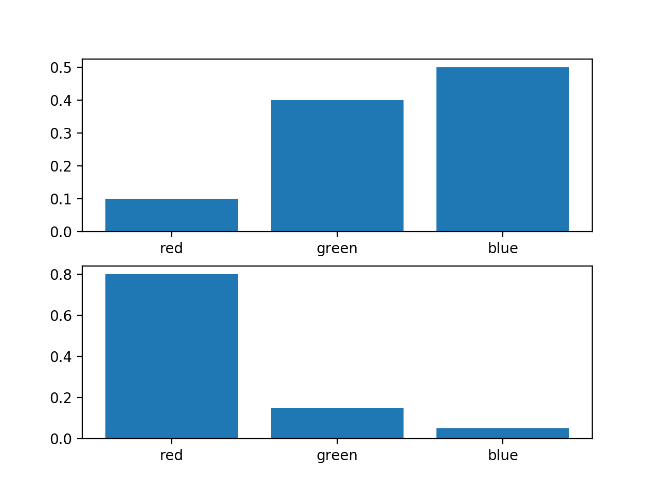
Histogram of Two Different Probability Distributions for the Same Random Variable
Next, we can develop a function to calculate the cross-entropy between the two distributions.
We will use log base-2 to ensure the result has units in bits.
# calculate cross entropy
def cross_entropy(p, q):
	return -sum([p[i]*log2(q[i]) for i in range(len(p))])
We can then use this function to calculate the cross-entropy of P from Q, as well as the reverse, Q from P.
...
# calculate cross entropy H(P, Q)
ce_pq = cross_entropy(p, q)
print('H(P, Q): %.3f bits' % ce_pq)
# calculate cross entropy H(Q, P)
ce_qp = cross_entropy(q, p)
print('H(Q, P): %.3f bits' % ce_qp)
Tying this all together, the complete example is listed below.
# example of calculating cross entropy
from math import log2

# calculate cross entropy
def cross_entropy(p, q):
	return -sum([p[i]*log2(q[i]) for i in range(len(p))])

# define data
p = [0.10, 0.40, 0.50]
q = [0.80, 0.15, 0.05]
# calculate cross entropy H(P, Q)
ce_pq = cross_entropy(p, q)
print('H(P, Q): %.3f bits' % ce_pq)
# calculate cross entropy H(Q, P)
ce_qp = cross_entropy(q, p)
print('H(Q, P): %.3f bits' % ce_qp)
Running the example first calculates the cross-entropy of Q from P as just over 3 bits, then P from Q as just under 3 bits.
H(P, Q): 3.288 bits
H(Q, P): 2.906 bits
We can also calculate the cross-entropy using the KL divergence.
The cross-entropy calculated with KL divergence should be identical, and it may be interesting to calculate the KL divergence between the distributions as well to see the relative entropy or additional bits required instead of the total bits calculated by the cross-entropy.
First, we can define a function to calculate the KL divergence between the distributions using log base-2 to ensure the result is also in bits.
# calculate the kl divergence KL(P || Q)
def kl_divergence(p, q):
	return sum(p[i] * log2(p[i]/q[i]) for i in range(len(p)))
Next, we can define a function to calculate the entropy for a given probability distribution.
# calculate entropy H(P)
def entropy(p):
	return -sum([p[i] * log2(p[i]) for i in range(len(p))])
Finally, we can calculate the cross-entropy using the entropy() and kl_divergence() functions.
# calculate cross entropy H(P, Q)
def cross_entropy(p, q):
	return entropy(p) + kl_divergence(p, q)
To keep the example simple, we can compare the cross-entropy for H(P, Q) to the KL divergence KL(P || Q) and the entropy H(P).
The complete example is listed below.
# example of calculating cross entropy with kl divergence
from math import log2

# calculate the kl divergence KL(P || Q)
def kl_divergence(p, q):
	return sum(p[i] * log2(p[i]/q[i]) for i in range(len(p)))

# calculate entropy H(P)
def entropy(p):
	return -sum([p[i] * log2(p[i]) for i in range(len(p))])

# calculate cross entropy H(P, Q)
def cross_entropy(p, q):
	return entropy(p) + kl_divergence(p, q)

# define data
p = [0.10, 0.40, 0.50]
q = [0.80, 0.15, 0.05]
# calculate H(P)
en_p = entropy(p)
print('H(P): %.3f bits' % en_p)
# calculate kl divergence KL(P || Q)
kl_pq = kl_divergence(p, q)
print('KL(P || Q): %.3f bits' % kl_pq)
# calculate cross entropy H(P, Q)
ce_pq = cross_entropy(p, q)
print('H(P, Q): %.3f bits' % ce_pq)
Running the example, we can see that the cross-entropy score of 3.288 bits is comprised of the entropy of P 1.361 and the additional 1.927 bits calculated by the KL divergence.
This is a useful example that clearly illustrates the relationship between all three calculations.
H(P): 1.361 bits
KL(P || Q): 1.927 bits
H(P, Q): 3.288 bits
Cross-Entropy as a Loss Function
Cross-entropy is widely used as a loss function when optimizing classification models.
Two examples that you may encounter include the logistic regression algorithm (a linear classification algorithm), and artificial neural networks that can be used for classification tasks.
… using the cross-entropy error function instead of the sum-of-squares for a classification problem leads to faster training as well as improved generalization.
— Page 235, Pattern Recognition and Machine Learning, 2006.
Classification problems are those that involve one or more input variables and the prediction of a class label. Classification tasks that have just two labels for the output variable are referred to as binary classification problems, whereas those problems with more than two labels are referred to as categorical or multi-class classification problems.
- Binary Classification: Task of predicting one of two class labels for a given example.
- Multi-Class Classification: Task of predicting one of more than two class labels for a given example.
We can see that the idea of cross-entropy may be useful for optimizing a classification model: that is, in calculating the difference between the probability distribution of class labels in the dataset and those predicted by the model.
In classification tasks, we do not have the target probability distribution P; instead, we must estimate it from the dataset. The predictions from the model represent the approximation of the target probability distribution Q. In the language of classification, these are the actual and the predicted probabilities, or y and yhat.
- Expected Probability (y): The probability of class labels taken from the dataset (P).
- Predicted Probability (yhat): The probability of class labels predicted by the model (Q).
We can, therefore, estimate the cross-entropy for a single prediction using the cross-entropy calculation described above; for example.
- H(P, Q) = – sum x in X P(x) * log(Q(x))
Where each x in X is a class label that could be assigned to the example, and P(x) will be 1 for the known label and 0 for all other labels.
If there are just two class labels, e.g. binary classification, then the probability for class 0 is predicted directly, and the probability for class 1 is given as one minus the probability. As such, the cross-entropy for a single example in a binary classification task can be stated by unrolling the sum operation as follows:
- H(P, Q) = – (P(class0) * log(Q(class0)) + P(class1) * log(Q(class1)))
You may see this form of calculating cross-entropy cited in textbooks.
When calculating cross-entropy for classification tasks, the base-e or natural logarithm is used. This means that the units are in nats, not bits.
We are often interested in minimizing the cross-entropy for the model across the entire training dataset. This is calculated by calculating the average cross-entropy across all training examples. As such, a cross-entropy of 0.0 indicates that the predicted probabilities from the model are identical to the probabilities in the training dataset, e.g. zero loss. In practice, a cross-entropy loss of 0.0 often indicates that the model has overfit the training dataset.
The use of cross-entropy for classification often gives different specific names based on the number of classes, mirroring the name of the classification task; for example:
- Binary Cross-Entropy: Cross-entropy as a loss function for a binary classification task.
- Categorical Cross-Entropy: Cross-entropy as a loss function for a multi-class classification task.
We can make the use of cross-entropy as a loss function concrete with a worked example.
Consider a binary classification task with the following 10 actual class labels (P) and predicted class labels (Q).
...
# define classification data
p = [1, 1, 1, 1, 1, 0, 0, 0, 0, 0]
q = [0.8, 0.9, 0.9, 0.6, 0.8, 0.1, 0.4, 0.2, 0.1, 0.3]
We can enumerate these probabilities and calculate the cross-entropy for each using the cross-entropy function developed in the previous section using log() (natural logarithm) instead of log2().
# calculate cross entropy
def cross_entropy(p, q):
	return -sum([p[i]*log(q[i]) for i in range(len(p))])
For each actual and predicted probability, we must convert the prediction into a distribution of probabilities across each state, in this case, the states {0, 1} as the probability and 1-probability.
We can then calculate the cross-entropy and repeat the process for all examples.
...
# calculate cross entropy for each example
results = list()
for i in range(len(p)):
	# create the distribution for each event {0, 1}
	expected = [p[i], 1.0 - p[i]]
	predicted = [q[i], 1.0 - q[i]]
	# calculate cross entropy for the two events
	ce = cross_entropy(expected, predicted)
	print('>[y=%.1f, yhat=%.1f] ce: %.3f nats' % (p[i], q[i], ce))
	results.append(ce)
Finally, we can calculate the average cross-entropy across the dataset and report it as the cross-entropy loss for the model on the dataset.
...
# calculate the average cross entropy
mean_ce = mean(results)
print('Average Cross Entropy: %.3f nats' % mean_ce)
Tying this all together, the complete example is listed below.
# calculate cross entropy for classification problem
from math import log
from numpy import mean

# calculate cross entropy
def cross_entropy(p, q):
	return -sum([p[i]*log(q[i]) for i in range(len(p))])

# define classification data
p = [1, 1, 1, 1, 1, 0, 0, 0, 0, 0]
q = [0.8, 0.9, 0.9, 0.6, 0.8, 0.1, 0.4, 0.2, 0.1, 0.3]
# calculate cross entropy for each example
results = list()
for i in range(len(p)):
	# create the distribution for each event {0, 1}
	expected = [p[i], 1.0 - p[i]]
	predicted = [q[i], 1.0 - q[i]]
	# calculate cross entropy for the two events
	ce = cross_entropy(expected, predicted)
	print('>[y=%.1f, yhat=%.1f] ce: %.3f nats' % (p[i], q[i], ce))
	results.append(ce)

# calculate the average cross entropy
mean_ce = mean(results)
print('Average Cross Entropy: %.3f nats' % mean_ce)
Running the example prints the actual and predicted probabilities for each example and the cross-entropy in nats.
The final average cross-entropy loss across all examples is reported, in this case, as 0.247 nats.
>[y=1.0, yhat=0.8] ce: 0.223 nats
>[y=1.0, yhat=0.9] ce: 0.105 nats
>[y=1.0, yhat=0.9] ce: 0.105 nats
>[y=1.0, yhat=0.6] ce: 0.511 nats
>[y=1.0, yhat=0.8] ce: 0.223 nats
>[y=0.0, yhat=0.1] ce: 0.105 nats
>[y=0.0, yhat=0.4] ce: 0.511 nats
>[y=0.0, yhat=0.2] ce: 0.223 nats
>[y=0.0, yhat=0.1] ce: 0.105 nats
>[y=0.0, yhat=0.3] ce: 0.357 nats
Average Cross Entropy: 0.247 nats
This is how cross-entropy loss is calculated when optimizing a logistic regression model or a neural network model under a cross-entropy loss function.
We can confirm this by using the binary_crossentropy() function from the Keras deep learning API to calculate the cross-entropy loss for our small dataset.
The complete example is listed below.
Note: This example assumes that you have the Keras library installed and configured with a backend library such as TensorFlow. If not, you can skip running this example.
# calculate cross entropy with keras
from numpy import asarray
from keras import backend
from keras.losses import binary_crossentropy
# prepare classification data
p = asarray([1, 1, 1, 1, 1, 0, 0, 0, 0, 0])
q = asarray([0.8, 0.9, 0.9, 0.6, 0.8, 0.1, 0.4, 0.2, 0.1, 0.3])
# convert to keras variables
y_true = backend.variable(p)
y_pred = backend.variable(q)
# calculate the average cross-entropy
mean_ce = backend.eval(binary_crossentropy(y_true, y_pred))
print('Average Cross Entropy: %.3f nats' % mean_ce)
Running the example, we can see that the same average cross-entropy loss of 0.247 nats is reported.
This confirms the correct manual calculation of cross-entropy.
Average Cross Entropy: 0.247 nats
We can see that we could just as easily minimize the KL divergence as a loss function instead of the cross-entropy. The specific values would be different, but the effect would be the same as the two values are proportional to each other (e.g. minus the constant of the entropy for P).
Minimizing this KL divergence corresponds exactly to minimizing the cross-entropy between the distributions.
— Page 132, Deep Learning, 2016.
Difference Between Cross-Entropy and Log Loss
Cross-Entropy is not Log Loss, but they calculate the same quantity when used as loss functions for binary classification problems.
Logistic loss refers to the loss function commonly used to optimize a logistic regression model.
It may also be referred to as logarithmic loss (which is confusing) or simply log loss.
Many models are optimized under a probabilistic framework called the maximum likelihood estimation, or MLE, that involves finding a set of parameters that best explain the observed data.
This involves selecting a likelihood function that defines how likely a set of observations (data) are given model parameters. When a log likelihood function is used (which is common), it is often referred to as optimizing the log likelihood for the model. Because it is more common to minimize a function than to maximize it in practice, the log likelihood function is inverted by adding a negative sign to the front. This transforms it into a Negative Log Likelihood function or NLL for short.
In deriving the log likelihood function under a framework of maximum likelihood estimation for Bernoulli probability distribution functions (two classes), the calculation comes out to be:
- negative log-likelihood(P, Q) = -(P(class0) * log(Q(class0)) + P(class1) * log(Q(class1)))
This quantity can be averaged over all training examples by calculating the average of the log of the likelihood function.
Negative log-likelihood for binary classification problems is often shortened to simply “log loss” as the loss function derived for logistic regression.
- log loss = negative log-likelihood, under a Bernoulli probability distribution
We can see that the negative log-likelihood is the same calculation as is used for the cross-entropy for Bernoulli probability distribution functions (two events or classes). In fact, the negative log-likelihood for Multinoulli distributions (multi-class classification) also matches the calculation for cross-entropy.
For binary classification problems, “log loss“, “cross-entropy” and “negative log-likelihood” are used interchangeably.
More generally, the terms “cross-entropy” and “negative log-likelihood” are used interchangeably in the context of loss functions for classification models.
The negative log-likelihood for logistic regression is given by […] This is also called the cross-entropy error function.
— Page 246, Machine Learning: A Probabilistic Perspective, 2012.
Therefore, calculating log loss will give the same quantity as calculating the cross-entropy for Bernoulli probability distribution. We can confirm this by calculating the log loss using the log_loss() function from the scikit-learn API.
Calculating the average log loss on the same set of actual and predicted probabilities from the previous section should give the same result as calculating the average cross-entropy.
The complete example is listed below.
# calculate log loss for classification problem with scikit-learn
from sklearn.metrics import log_loss
from numpy import asarray
# define classification data
p = [1, 1, 1, 1, 1, 0, 0, 0, 0, 0]
q = [0.8, 0.9, 0.9, 0.6, 0.8, 0.1, 0.4, 0.2, 0.1, 0.3]
# define data as expected, e.g. probability for each event {0, 1}
y_true = asarray([[v, 1-v] for v in p])
y_pred = asarray([[v, 1-v] for v in q])
# calculate the average log loss
ll = log_loss(y_true, y_pred)
print('Average Log Loss: %.3f' % ll)
Running the example gives the expected result of 0.247 log loss, which matches 0.247 nats when calculated using the average cross-entropy.
Average Log Loss: 0.247
This does not mean that log loss calculates cross-entropy or cross-entropy calculates log loss.
Instead, they are different quantities, arrived at from different fields of study, that under the conditions of calculating a loss function for a classification task, result in an equivalent calculation and result. Specifically, a cross-entropy loss function is equivalent to a maximum likelihood function under a Bernoulli or Multinoulli probability distribution.
More generally, a cross-entropy for a continuous probability distribution such as a Gaussian is equivalent to the mean squared error likelihood function.
Any loss consisting of a negative log-likelihood is a cross- entropy between the empirical distribution defined by the training set and the probability distribution defined by model. For example, mean squared error is the cross-entropy between the empirical distribution and a Gaussian model.
— Page 132, Deep Learning, 2016.
Further Reading
This section provides more resources on the topic if you are looking to go deeper.
Posts
- How to Choose Loss Functions When Training Deep Learning Neural Networks
- Loss and Loss Functions for Training Deep Learning Neural Networks
Books
- Machine Learning: A Probabilistic Perspective, 2012.
- Pattern Recognition and Machine Learning, 2006.
- Deep Learning, 2016.
API
Articles
- Kullback-Leibler divergence, Wikipedia.
- Cross entropy, Wikipedia.
- Joint Entropy, Wikipedia.
- Loss functions for classification, Wikipedia.
Summary
In this tutorial, you discovered cross-entropy for machine learning.
Specifically, you learned:
- How to calculate cross-entropy from scratch and using standard machine learning libraries.
- Cross-entropy can be used as a loss function when optimizing classification models like logistic regression and artificial neural networks.
- Cross-entropy is different from KL divergence but can be calculated using KL divergence, and is different from log loss but calculates the same quantity when used as a loss function.
Do you have any questions?
Ask your questions in the comments below and I will do my best to answer.
The post A Gentle Introduction to Cross-Entropy for Machine Learning appeared first on Machine Learning Mastery.