
Author: Jason Brownlee
An empirical distribution function provides a way to model and sample cumulative probabilities for a data sample that does not fit a standard probability distribution.
As such, it is sometimes called the empirical cumulative distribution function, or ECDF for short.
In this tutorial, you will discover the empirical probability distribution function.
After completing this tutorial, you will know:
- Some data samples cannot be summarized using a standard distribution.
- An empirical distribution function provides a way of modeling cumulative probabilities for a data sample.
- How to use the statsmodels library to model and sample an empirical cumulative distribution function.
Discover bayes opimization, naive bayes, maximum likelihood, distributions, cross entropy, and much more in my new book, with 28 step-by-step tutorials and full Python source code.
Let’s get started.

How to Use an Empirical Distribution Function in Python
Photo by Gigi Griffis, some rights reserved.
Tutorial Overview
This tutorial is divided into three parts; they are:
- Empirical Distribution Function
- Bimodal Data Distribution
- Sampling Empirical Distribution
Empirical Distribution Function
Typically, the distribution of observations for a data sample fits a well-known probability distribution.
For example, the heights of humans will fit the normal (Gaussian) probability distribution.
This is not always the case. Sometimes the observations in a collected data sample do not fit any known probability distribution and cannot be easily forced into an existing distribution by data transforms or parameterization of the distribution function.
Instead, an empirical probability distribution must be used.
There are two main types of probability distribution functions we may need to sample; they are:
- Probability Density Function (PDF).
- Cumulative Distribution Function (CDF).
The PDF returns the expected probability for observing a value. For discrete data, the PDF is referred to as a Probability Mass Function (PMF). The CDF returns the expected probability for observing a value less than or equal to a given value.
An empirical probability density function can be fit and used for a data sampling using a nonparametric density estimation method, such as Kernel Density Estimation (KDE).
An empirical cumulative distribution function is called the Empirical Distribution Function, or EDF for short. It is also referred to as the Empirical Cumulative Distribution Function, or ECDF.
The EDF is calculated by ordering all of the unique observations in the data sample and calculating the cumulative probability for each as the number of observations less than or equal to a given observation divided by the total number of observations.
As follows:
- EDF(x) = number of observations <= x / n
Like other cumulative distribution functions, the sum of probabilities will proceed from 0.0 to 1.0 as the observations in the domain are enumerated from smallest to largest.
To make the empirical distribution function concrete, let’s look at an example with a dataset that clearly does not fit a known probability distribution.
Want to Learn Probability for Machine Learning
Take my free 7-day email crash course now (with sample code).
Click to sign-up and also get a free PDF Ebook version of the course.
Bimodal Data Distribution
We can define a dataset that clearly does not match a standard probability distribution function.
A common example is when the data has two peaks (bimodal distribution) or many peaks (multimodal distribution).
We can construct a bimodal distribution by combining samples from two different normal distributions. Specifically, 300 examples with a mean of 20 and a standard deviation of five (the smaller peak), and 700 examples with a mean of 40 and a standard deviation of five (the larger peak).
The means were chosen close together to ensure the distributions overlap in the combined sample.
The complete example of creating this sample with a bimodal probability distribution and plotting the histogram is listed below.
# example of a bimodal data sample
from matplotlib import pyplot
from numpy.random import normal
from numpy import hstack
# generate a sample
sample1 = normal(loc=20, scale=5, size=300)
sample2 = normal(loc=40, scale=5, size=700)
sample = hstack((sample1, sample2))
# plot the histogram
pyplot.hist(sample, bins=50)
pyplot.show()
Running the example creates the data sample and plots the histogram.
Note that your results will differ given the random nature of the data sample. Try running the example a few times.
We have fewer samples with a mean of 20 than samples with a mean of 40, which we can see reflected in the histogram with a larger density of samples around 40 than around 20.
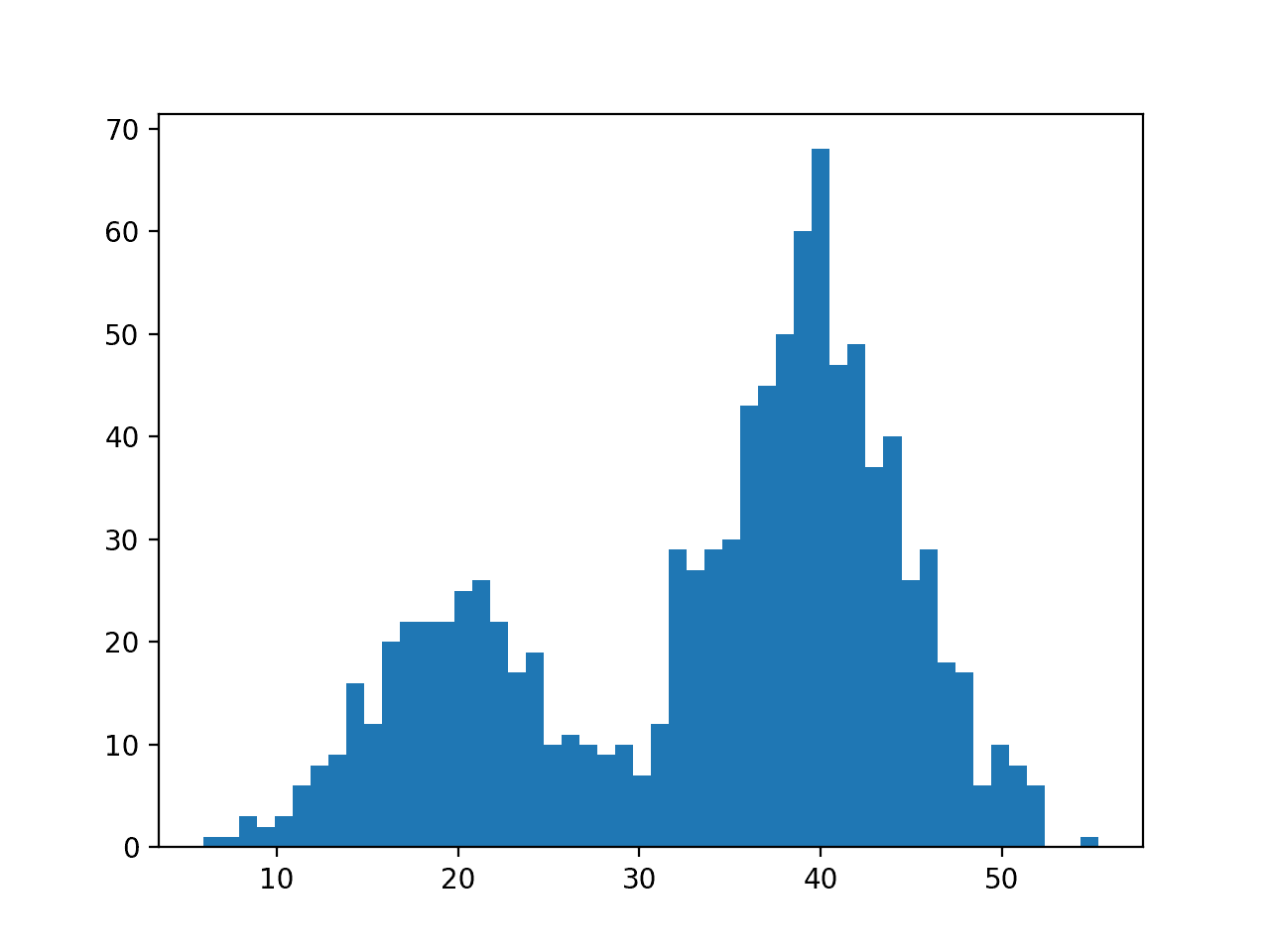
Histogram Plot of Data Sample With a Bimodal Probability Distribution
Data with this distribution does not nicely fit into a common probability distribution by design.
Below is a plot of the probability density function (PDF) of this data sample.
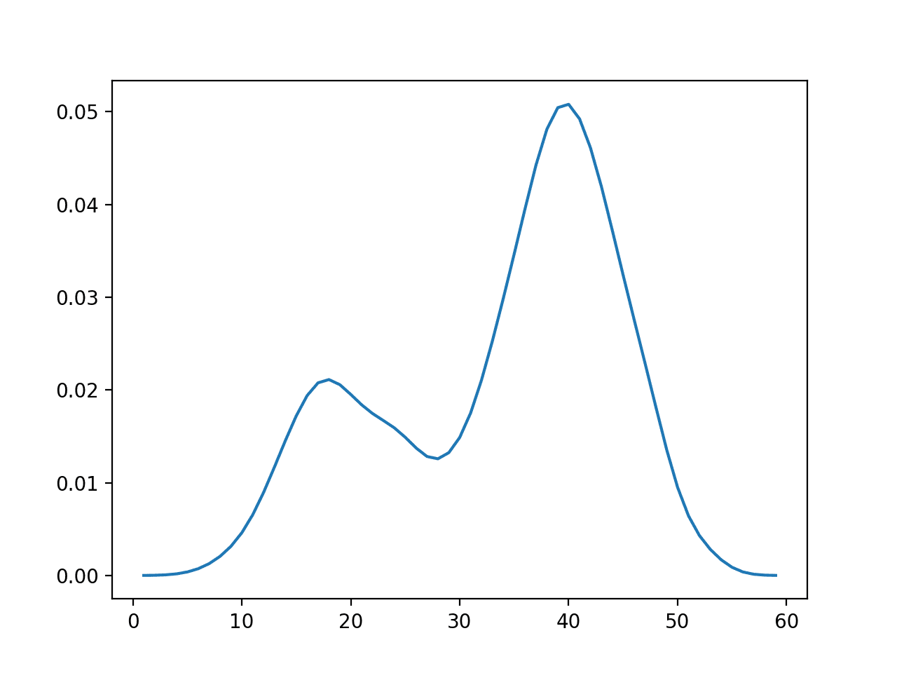
Empirical Probability Density Function for the Bimodal Data Sample
It is a good case for using an empirical distribution function.
Calculate the Empirical Distribution Function
An empirical distribution function can be fit for a data sample in Python.
The statmodels Python library provides the ECDF class for fitting an empirical cumulative distribution function and calculating the cumulative probabilities for specific observations from the domain.
The distribution is fit by calling ECDF() and passing in the raw data sample.
...
# fit a cdf
ecdf = ECDF(sample)
Once fit, the function can be called to calculate the cumulative probability for a given observation.
...
# get cumulative probability for values
print('P(x<20): %.3f' % ecdf(20))
print('P(x<40): %.3f' % ecdf(40))
print('P(x<60): %.3f' % ecdf(60))
The class also provides an ordered list of unique observations in the data (the .x attribute) and their associated probabilities (.y attribute). We can access these attributes and plot the CDF function directly.
...
# plot the cdf
pyplot.plot(ecdf.x, ecdf.y)
pyplot.show()
Tying this together, the complete example of fitting an empirical distribution function for the bimodal data sample is below.
# fit an empirical cdf to a bimodal dataset
from matplotlib import pyplot
from numpy.random import normal
from numpy import hstack
from statsmodels.distributions.empirical_distribution import ECDF
# generate a sample
sample1 = normal(loc=20, scale=5, size=300)
sample2 = normal(loc=40, scale=5, size=700)
sample = hstack((sample1, sample2))
# fit a cdf
ecdf = ECDF(sample)
# get cumulative probability for values
print('P(x<20): %.3f' % ecdf(20))
print('P(x<40): %.3f' % ecdf(40))
print('P(x<60): %.3f' % ecdf(60))
# plot the cdf
pyplot.plot(ecdf.x, ecdf.y)
pyplot.show()
Running the example fits the empirical CDF to the data sample, then prints the cumulative probability for observing three values.
Your specific results will vary given the stochastic nature of the data sample. Try running the example a few times.
P(x<20): 0.149
P(x<40): 0.654
P(x<60): 1.000
Then the cumulative probability for the entire domain is calculated and shown as a line plot.
Here, we can see the familiar S-shaped curve seen for most cumulative distribution functions, here with bumps around the mean of both peaks of the bimodal distribution.
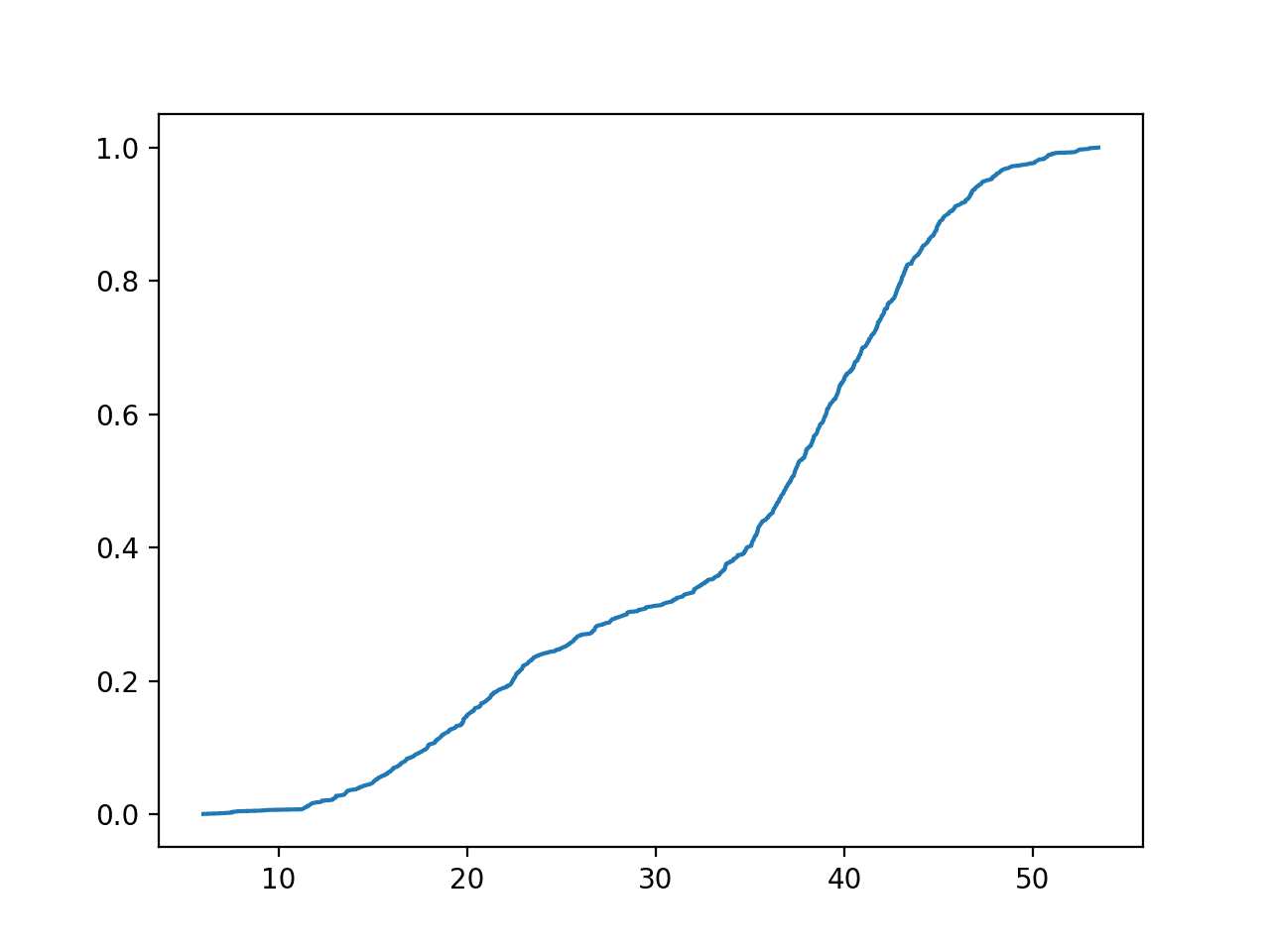
Empirical Cumulative Distribution Function for the Bimodal Data Sample
Further Reading
This section provides more resources on the topic if you are looking to go deeper.
Books
- Section 2.3.4 The empirical distribution, Machine Learning: A Probabilistic Perspective, 2012.
- Section 3.9.5 The Dirac Distribution and Empirical Distribution, Deep Learning, 2016.
API
Articles
- Empirical distribution function, Wikipedia.
- Cumulative distribution function, Wikipedia.
- Probability Density Function, Wikipedia.
- Kernel density estimation, Wikipedia.
Summary
In this tutorial, you discovered the empirical probability distribution function.
Specifically, you learned:
- Some data samples cannot be summarized using a standard distribution.
- An empirical distribution function provides a way of modeling cumulative probabilities for a data sample.
- How to use the statsmodels library to model and sample an empirical cumulative distribution function.
Do you have any questions?
Ask your questions in the comments below and I will do my best to answer.
The post How to Use an Empirical Distribution Function in Python appeared first on Machine Learning Mastery.