
Author: Jason Brownlee
Selecting a machine learning algorithm for a predictive modeling problem involves evaluating many different models and model configurations using k-fold cross-validation.
The super learner is an ensemble machine learning algorithm that combines all of the models and model configurations that you might investigate for a predictive modeling problem and uses them to make a prediction as-good-as or better than any single model that you may have investigated.
The super learner algorithm is an application of stacked generalization, called stacking or blending, to k-fold cross-validation where all models use the same k-fold splits of the data and a meta-model is fit on the out-of-fold predictions from each model.
In this tutorial, you will discover the super learner ensemble machine learning algorithm.
After completing this tutorial, you will know:
- Super learner is the application of stacked generalization using out-of-fold predictions during k-fold cross-validation.
- The super learner ensemble algorithm is straightforward to implement in Python using scikit-learn models.
- The ML-Ensemble (mlens) library provides a convenient implementation that allows the super learner to be fit and used in just a few lines of code.
Let’s get started.

How to Develop Super Learner Ensembles in Python
Photo by Mark Gunn, some rights reserved.
Tutorial Overview
This tutorial is divided into three parts; they are:
- What Is the Super Learner?
- Manually Develop a Super Learner With scikit-learn
- Super Learner With ML-Ensemble Library
What Is the Super Learner?
There are many hundreds of models to choose from for a predictive modeling problem; which one is best?
Then, after a model is chosen, how do you best configure it for your specific dataset?
These are open questions in applied machine learning. The best answer we have at the moment is to use empirical experimentation to test and discover what works best for your dataset.
In practice, it is generally impossible to know a priori which learner will perform best for a given prediction problem and data set.
— Super Learner, 2007.
This involves selecting many different algorithms that may be appropriate for your regression or classification problem and evaluating their performance on your dataset using a resampling technique, such as k-fold cross-validation.
The algorithm that performs the best on your dataset according to k-fold cross-validation is then selected, fit on all available data, and you can then start using it to make predictions.
There is an alternative approach.
Consider that you have already fit many different algorithms on your dataset, and some algorithms have been evaluated many times with different configurations. You may have many tens or hundreds of different models of your problem. Why not use all those models instead of the best model from the group?
This is the intuition behind the so-called “super learner” ensemble algorithm.
The super learner algorithm involves first pre-defining the k-fold split of your data, then evaluating all different algorithms and algorithm configurations on the same split of the data. All out-of-fold predictions are then kept and used to train a that learns how to best combine the predictions.
The algorithms may differ in the subset of the covariates used, the basis functions, the loss functions, the searching algorithm, and the range of tuning parameters, among others.
— Super Learner In Prediction, 2010.
The results of this model should be no worse than the best performing model evaluated during k-fold cross-validation and has the likelihood of performing better than any single model.
The super learner algorithm was proposed by Mark van der Laan, Eric Polley, and Alan Hubbard from Berkeley in their 2007 paper titled “Super Learner.” It was published in a biological journal, which may be sheltered from the broader machine learning community.
The super learner technique is an example of the general method called “stacked generalization,” or “stacking” for short, and is known in applied machine learning as blending, as often a linear model is used as the meta-model.
The super learner is related to the stacking algorithm introduced in neural networks context …
— Super Learner In Prediction, 2010.
For more on the topic stacking, see the posts:
- How to Develop a Stacking Ensemble for Deep Learning Neural Networks in Python With Keras
- How to Implement Stacked Generalization (Stacking) From Scratch With Python
We can think of the “super learner” as the supplicating of stacking specifically to k-fold cross-validation.
I have sometimes seen this type of blending ensemble referred to as a cross-validation ensemble.
The procedure can be summarized as follows:
- 1. Select a k-fold split of the training dataset.
- 2. Select m base-models or model configurations.
- 3. For each basemodel:
- a. Evaluate using k-fold cross-validation.
- b. Store all out-of-fold predictions.
- c. Fit the model on the full training dataset and store.
- 4. Fit a meta-model on the out-of-fold predictions.
- 5. Evaluate the model on a holdout dataset or use model to make predictions.
The image below, taken from the original paper, summarizes this data flow.
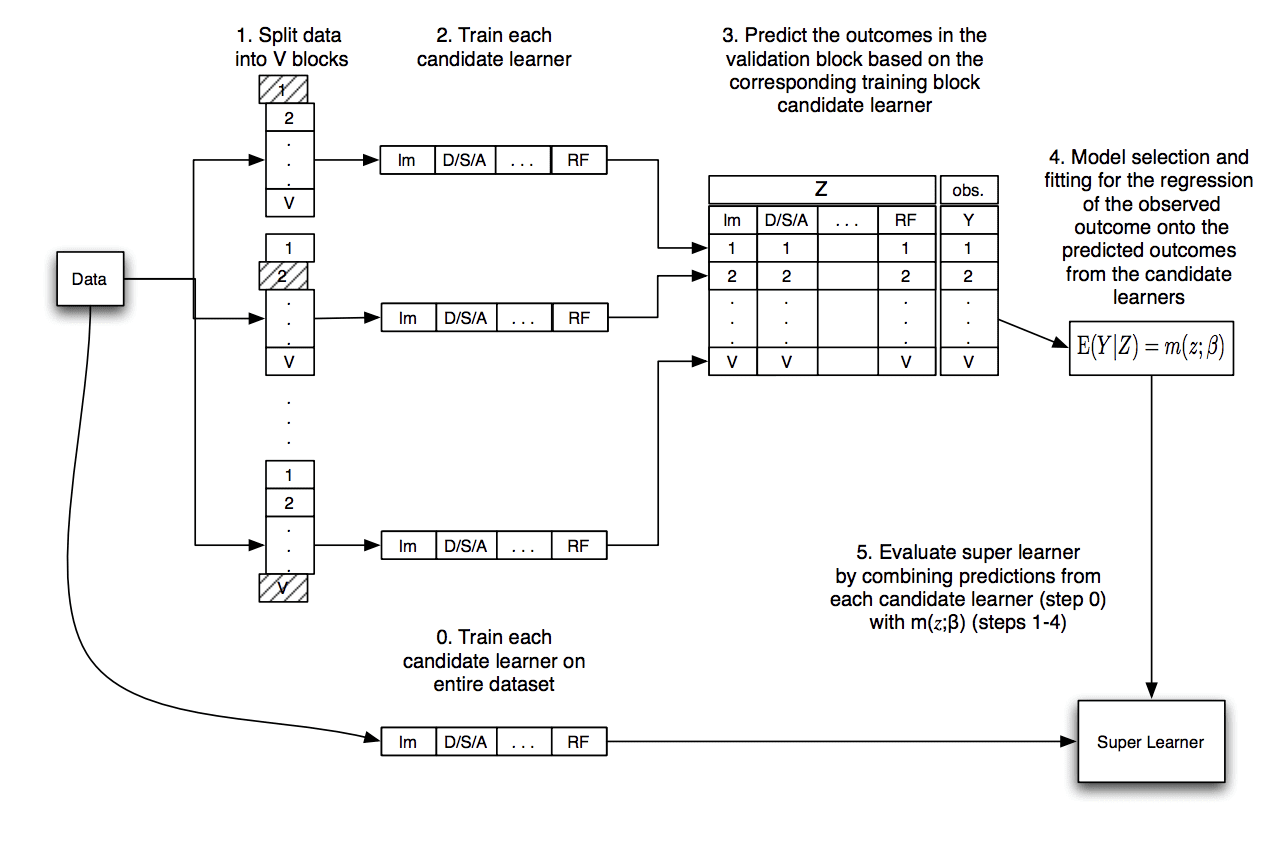
Diagram Showing the Data Flow of the Super Learner Algorithm
Taken from “Super Learner.”
Let’s take a closer look at some common sticking points you may have with this procedure.
Q. What are the inputs and outputs for the meta-model?
The meta-model takes in predictions from base-models as input and predicts the target for the training dataset as output:
- Input: Predictions from base-models.
- Output: Prediction for training dataset.
For example, if we had 50 base-models, then one input sample would be a vector with 50 values, each value in the vector representing a prediction from one of the base-models for one sample of the training dataset.
If we had 1,000 examples (rows) in the training dataset and 50 models, then the input data for the meta-model would be 1,000 rows and 50 columns.
Q. Won’t the meta-model overfit the training data?
Probably not.
This is the trick of the super learner, and the stacked generalization procedure in general.
The input to the meta-model is the out-of-fold (out-of-sample) predictions. In aggregate, the out-of-fold predictions for a model represent the model’s skill or capability in making predictions on data not seen during training.
By training a meta-model on out-of-sample predictions of other models, the meta-model learns how to both correct the out-of-sample predictions for each model and to best combine the out-of-sample predictions from multiple models; actually, it does both tasks at the same time.
Importantly, to get an idea of the true capability of the meta-model, it must be evaluated on new out-of-sample data. That is, data not used to train the base models.
Q. Can this work for regression and classification?
Yes, it was described in the papers for regression (predicting a numerical value).
It can work just as well for classification (predicting a class label), although it is probably best to predict probabilities to give the meta-model more granularity when combining predictions.
Q. Why do we fit each base-model on the entire training dataset?
Each base-model is fit on the entire training dataset so that the model can be used later to make predictions on new examples not seen during training.
This step is strictly not required until predictions are needed by the super learner.
Q. How do we make a prediction?
To make a prediction on a new sample (row of data), first, the row of data is provided as input to each base model to generate a prediction from each model.
The predictions from the base-models are then concatenated into a vector and provided as input to the meta-model. The meta-model then makes a final prediction for the row of data.
We can summarize this procedure as follows:
- 1. Take a sample not seen by the models during training.
- 2. For each base-model:
- a. Make a prediction given the sample.
- b. Store prediction.
- 3. Concatenate predictions from submodel into a single vector.
- 4. Provide vector as input to the meta-model to make a final prediction.
Now that we are familiar with the super learner algorithm, let’s look at a worked example.
Manually Develop a Super Learner With scikit-learn
The Super Learner algorithm is relatively straightforward to implement on top of the scikit-learn Python machine learning library.
In this section, we will develop an example of super learning for both regression and classification that you can adapt to your own problems.
Super Learner for Regression
We will use the make_regression() test problem and generate 1,000 examples (rows) with 100 features (columns). This is a simple regression problem with a linear relationship between input and output, with added noise.
We will split the data so that 50 percent is used for training the model and 50 percent is held back to evaluate the final super model and base-models.
...
# create the inputs and outputs
X, y = make_regression(n_samples=1000, n_features=100, noise=0.5)
# split
X, X_val, y, y_val = train_test_split(X, y, test_size=0.50)
print('Train', X.shape, y.shape, 'Test', X_val.shape, y_val.shape)
Next, we will define a bunch of different regression models.
In this case, we will use nine different algorithms with modest configuration. You can use any models or model configurations you like.
The get_models() function below defines all of the models and returns them as a list.
# create a list of base-models
def get_models():
	models = list()
	models.append(LinearRegression())
	models.append(ElasticNet())
	models.append(SVR(gamma='scale'))
	models.append(DecisionTreeRegressor())
	models.append(KNeighborsRegressor())
	models.append(AdaBoostRegressor())
	models.append(BaggingRegressor(n_estimators=10))
	models.append(RandomForestRegressor(n_estimators=10))
	models.append(ExtraTreesRegressor(n_estimators=10))
	return models
Next, we will use k-fold cross-validation to make out-of-fold predictions that will be used as the dataset to train the meta-model or “super learner.”
This involves first splitting the data into k folds; we will use 10. For each fold, we will fit the model on the training part of the split and make out-of-fold predictions on the test part of the split. This is repeated for each model and all out-of-fold predictions are stored.
Each out-of-fold prediction will be a column for the meta-model input. We will collect columns from each algorithm for one fold of the data, horizontally stacking the rows. Then for all groups of columns we collect, we will vertically stack these rows into one long dataset with 500 rows and nine columns.
The get_out_of_fold_predictions() function below does this for a given test dataset and list of models; it will return the input and output dataset required to train the meta-model.
# collect out of fold predictions form k-fold cross validation
def get_out_of_fold_predictions(X, y, models):
	meta_X, meta_y = list(), list()
	# define split of data
	kfold = KFold(n_splits=10, shuffle=True)
	# enumerate splits
	for train_ix, test_ix in kfold.split(X):
		fold_yhats = list()
		# get data
		train_X, test_X = X[train_ix], X[test_ix]
		train_y, test_y = y[train_ix], y[test_ix]
		meta_y.extend(test_y)
		# fit and make predictions with each sub-model
		for model in models:
			model.fit(train_X, train_y)
			yhat = model.predict(test_X)
			# store columns
			fold_yhats.append(yhat.reshape(len(yhat),1))
		# store fold yhats as columns
		meta_X.append(hstack(fold_yhats))
	return vstack(meta_X), asarray(meta_y)
We can then call the function to get the models and the function to prepare the meta-model dataset.
...
# get models
models = get_models()
# get out of fold predictions
meta_X, meta_y = get_out_of_fold_predictions(X, y, models)
print('Meta ', meta_X.shape, meta_y.shape)
Next, we can fit all of the base-models on the entire training dataset.
# fit all base models on the training dataset
def fit_base_models(X, y, models):
	for model in models:
		model.fit(X, y)
Then, we can fit the meta-model on the prepared dataset.
In this case, we will use a linear regression model as the meta-model, as was used in the original paper.
# fit a meta model
def fit_meta_model(X, y):
	model = LinearRegression()
	model.fit(X, y)
	return model
Next, we can evaluate the base-models on the holdout dataset.
# evaluate a list of models on a dataset
def evaluate_models(X, y, models):
	for model in models:
		yhat = model.predict(X)
		mse = mean_squared_error(y, yhat)
		print('%s: RMSE %.3f' % (model.__class__.__name__, sqrt(mse)))
And, finally, use the super learner (base and meta-model) to make predictions on the holdout dataset and evaluate the performance of the approach.
The super_learner_predictions() function below will use the meta-model to make predictions for new data.
# make predictions with stacked model
def super_learner_predictions(X, models, meta_model):
	meta_X = list()
	for model in models:
		yhat = model.predict(X)
		meta_X.append(yhat.reshape(len(yhat),1))
	meta_X = hstack(meta_X)
	# predict
	return meta_model.predict(meta_X)
We can call this function and evaluate the results.
...
# evaluate meta model
yhat = super_learner_predictions(X_val, models, meta_model)
print('Super Learner: RMSE %.3f' % (sqrt(mean_squared_error(y_val, yhat))))
Tying this all together, the complete example of a super learner algorithm for regression using scikit-learn models is listed below.
# example of a super learner model for regression
from math import sqrt
from numpy import hstack
from numpy import vstack
from numpy import asarray
from sklearn.datasets.samples_generator import make_regression
from sklearn.model_selection import KFold
from sklearn.model_selection import train_test_split
from sklearn.metrics import mean_squared_error
from sklearn.linear_model import LinearRegression
from sklearn.linear_model import ElasticNet
from sklearn.neighbors import KNeighborsRegressor
from sklearn.tree import DecisionTreeRegressor
from sklearn.svm import SVR
from sklearn.ensemble import AdaBoostRegressor
from sklearn.ensemble import BaggingRegressor
from sklearn.ensemble import RandomForestRegressor
from sklearn.ensemble import ExtraTreesRegressor

# create a list of base-models
def get_models():
	models = list()
	models.append(LinearRegression())
	models.append(ElasticNet())
	models.append(SVR(gamma='scale'))
	models.append(DecisionTreeRegressor())
	models.append(KNeighborsRegressor())
	models.append(AdaBoostRegressor())
	models.append(BaggingRegressor(n_estimators=10))
	models.append(RandomForestRegressor(n_estimators=10))
	models.append(ExtraTreesRegressor(n_estimators=10))
	return models

# collect out of fold predictions form k-fold cross validation
def get_out_of_fold_predictions(X, y, models):
	meta_X, meta_y = list(), list()
	# define split of data
	kfold = KFold(n_splits=10, shuffle=True)
	# enumerate splits
	for train_ix, test_ix in kfold.split(X):
		fold_yhats = list()
		# get data
		train_X, test_X = X[train_ix], X[test_ix]
		train_y, test_y = y[train_ix], y[test_ix]
		meta_y.extend(test_y)
		# fit and make predictions with each sub-model
		for model in models:
			model.fit(train_X, train_y)
			yhat = model.predict(test_X)
			# store columns
			fold_yhats.append(yhat.reshape(len(yhat),1))
		# store fold yhats as columns
		meta_X.append(hstack(fold_yhats))
	return vstack(meta_X), asarray(meta_y)

# fit all base models on the training dataset
def fit_base_models(X, y, models):
	for model in models:
		model.fit(X, y)

# fit a meta model
def fit_meta_model(X, y):
	model = LinearRegression()
	model.fit(X, y)
	return model

# evaluate a list of models on a dataset
def evaluate_models(X, y, models):
	for model in models:
		yhat = model.predict(X)
		mse = mean_squared_error(y, yhat)
		print('%s: RMSE %.3f' % (model.__class__.__name__, sqrt(mse)))

# make predictions with stacked model
def super_learner_predictions(X, models, meta_model):
	meta_X = list()
	for model in models:
		yhat = model.predict(X)
		meta_X.append(yhat.reshape(len(yhat),1))
	meta_X = hstack(meta_X)
	# predict
	return meta_model.predict(meta_X)

# create the inputs and outputs
X, y = make_regression(n_samples=1000, n_features=100, noise=0.5)
# split
X, X_val, y, y_val = train_test_split(X, y, test_size=0.50)
print('Train', X.shape, y.shape, 'Test', X_val.shape, y_val.shape)
# get models
models = get_models()
# get out of fold predictions
meta_X, meta_y = get_out_of_fold_predictions(X, y, models)
print('Meta ', meta_X.shape, meta_y.shape)
# fit base models
fit_base_models(X, y, models)
# fit the meta model
meta_model = fit_meta_model(meta_X, meta_y)
# evaluate base models
evaluate_models(X_val, y_val, models)
# evaluate meta model
yhat = super_learner_predictions(X_val, models, meta_model)
print('Super Learner: RMSE %.3f' % (sqrt(mean_squared_error(y_val, yhat))))
Running the example first reports the shape of the prepared dataset, then the shape of the dataset for the meta-model.
Next, the performance of each base-model is reported on the holdout dataset, and finally, the performance of the super learner on the holdout dataset.
Your specific results will differ given the stochastic nature of the dataset and learning algorithms. Try running the example a few times.
In this case, we can see that the linear models perform well on the dataset and the nonlinear algorithms not so well.
We can also see that the super learner out-performed all of the base-models.
Train (500, 100) (500,) Test (500, 100) (500,)
Meta  (500, 9) (500,)

LinearRegression: RMSE 0.548
ElasticNet: RMSE 67.142
SVR: RMSE 172.717
DecisionTreeRegressor: RMSE 159.137
KNeighborsRegressor: RMSE 154.064
AdaBoostRegressor: RMSE 98.422
BaggingRegressor: RMSE 108.915
RandomForestRegressor: RMSE 115.637
ExtraTreesRegressor: RMSE 105.749

Super Learner: RMSE 0.546
You can imagine plugging in all kinds of different models into this example, including XGBoost and Keras deep learning models.
Now that we have seen how to develop a super learner for regression, let’s look at an example for classification.
Super Learner for Classification
The super learner algorithm for classification is much the same.
The inputs to the meta learner can be class labels or class probabilities, with the latter more likely to be useful given the increased granularity or uncertainty captured in the predictions.
In this problem, we will use the make_blobs() test classification problem and use 1,000 examples with 100 input variables and two class labels.
...
# create the inputs and outputs
X, y = make_blobs(n_samples=1000, centers=2, n_features=100, cluster_std=20)
# split
X, X_val, y, y_val = train_test_split(X, y, test_size=0.50)
print('Train', X.shape, y.shape, 'Test', X_val.shape, y_val.shape)
Next, we can change the get_models() function to define a suite of linear and nonlinear classification algorithms.
# create a list of base-models
def get_models():
	models = list()
	models.append(LogisticRegression(solver='liblinear'))
	models.append(DecisionTreeClassifier())
	models.append(SVC(gamma='scale', probability=True))
	models.append(GaussianNB())
	models.append(KNeighborsClassifier())
	models.append(AdaBoostClassifier())
	models.append(BaggingClassifier(n_estimators=10))
	models.append(RandomForestClassifier(n_estimators=10))
	models.append(ExtraTreesClassifier(n_estimators=10))
	return models
Next, we can change the get_out_of_fold_predictions() function to predict probabilities by a call to the predict_proba() function.
# collect out of fold predictions form k-fold cross validation
def get_out_of_fold_predictions(X, y, models):
	meta_X, meta_y = list(), list()
	# define split of data
	kfold = KFold(n_splits=10, shuffle=True)
	# enumerate splits
	for train_ix, test_ix in kfold.split(X):
		fold_yhats = list()
		# get data
		train_X, test_X = X[train_ix], X[test_ix]
		train_y, test_y = y[train_ix], y[test_ix]
		meta_y.extend(test_y)
		# fit and make predictions with each sub-model
		for model in models:
			model.fit(train_X, train_y)
			yhat = model.predict_proba(test_X)
			# store columns
			fold_yhats.append(yhat)
		# store fold yhats as columns
		meta_X.append(hstack(fold_yhats))
	return vstack(meta_X), asarray(meta_y)
A Logistic Regression algorithm instead of a Linear Regression algorithm will be used as the meta-algorithm in the fit_meta_model() function.
# fit a meta model
def fit_meta_model(X, y):
	model = LogisticRegression(solver='liblinear')
	model.fit(X, y)
	return model
And classification accuracy will be used to report model performance.
The complete example of the super learner algorithm for classification using scikit-learn models is listed below.
# example of a super learner model for binary classification
from numpy import hstack
from numpy import vstack
from numpy import asarray
from sklearn.datasets.samples_generator import make_blobs
from sklearn.model_selection import KFold
from sklearn.model_selection import train_test_split
from sklearn.metrics import accuracy_score
from sklearn.neighbors import KNeighborsClassifier
from sklearn.linear_model import LogisticRegression
from sklearn.tree import DecisionTreeClassifier
from sklearn.svm import SVC
from sklearn.naive_bayes import GaussianNB
from sklearn.ensemble import AdaBoostClassifier
from sklearn.ensemble import BaggingClassifier
from sklearn.ensemble import RandomForestClassifier
from sklearn.ensemble import ExtraTreesClassifier

# create a list of base-models
def get_models():
	models = list()
	models.append(LogisticRegression(solver='liblinear'))
	models.append(DecisionTreeClassifier())
	models.append(SVC(gamma='scale', probability=True))
	models.append(GaussianNB())
	models.append(KNeighborsClassifier())
	models.append(AdaBoostClassifier())
	models.append(BaggingClassifier(n_estimators=10))
	models.append(RandomForestClassifier(n_estimators=10))
	models.append(ExtraTreesClassifier(n_estimators=10))
	return models

# collect out of fold predictions form k-fold cross validation
def get_out_of_fold_predictions(X, y, models):
	meta_X, meta_y = list(), list()
	# define split of data
	kfold = KFold(n_splits=10, shuffle=True)
	# enumerate splits
	for train_ix, test_ix in kfold.split(X):
		fold_yhats = list()
		# get data
		train_X, test_X = X[train_ix], X[test_ix]
		train_y, test_y = y[train_ix], y[test_ix]
		meta_y.extend(test_y)
		# fit and make predictions with each sub-model
		for model in models:
			model.fit(train_X, train_y)
			yhat = model.predict_proba(test_X)
			# store columns
			fold_yhats.append(yhat)
		# store fold yhats as columns
		meta_X.append(hstack(fold_yhats))
	return vstack(meta_X), asarray(meta_y)

# fit all base models on the training dataset
def fit_base_models(X, y, models):
	for model in models:
		model.fit(X, y)

# fit a meta model
def fit_meta_model(X, y):
	model = LogisticRegression(solver='liblinear')
	model.fit(X, y)
	return model

# evaluate a list of models on a dataset
def evaluate_models(X, y, models):
	for model in models:
		yhat = model.predict(X)
		acc = accuracy_score(y, yhat)
		print('%s: %.3f' % (model.__class__.__name__, acc*100))

# make predictions with stacked model
def super_learner_predictions(X, models, meta_model):
	meta_X = list()
	for model in models:
		yhat = model.predict_proba(X)
		meta_X.append(yhat)
	meta_X = hstack(meta_X)
	# predict
	return meta_model.predict(meta_X)

# create the inputs and outputs
X, y = make_blobs(n_samples=1000, centers=2, n_features=100, cluster_std=20)
# split
X, X_val, y, y_val = train_test_split(X, y, test_size=0.50)
print('Train', X.shape, y.shape, 'Test', X_val.shape, y_val.shape)
# get models
models = get_models()
# get out of fold predictions
meta_X, meta_y = get_out_of_fold_predictions(X, y, models)
print('Meta ', meta_X.shape, meta_y.shape)
# fit base models
fit_base_models(X, y, models)
# fit the meta model
meta_model = fit_meta_model(meta_X, meta_y)
# evaluate base models
evaluate_models(X_val, y_val, models)
# evaluate meta model
yhat = super_learner_predictions(X_val, models, meta_model)
print('Super Learner: %.3f' % (accuracy_score(y_val, yhat) * 100))
As before, the shape of the dataset and the prepared meta dataset is reported, followed by the performance of the base-models on the holdout dataset and finally the super model itself on the holdout dataset.
Your specific results will differ given the stochastic nature of the dataset and learning algorithms. Try running the example a few times.
In this case, we can see that the super learner has slightly better performance than the base learner algorithms.
Train (500, 100) (500,) Test (500, 100) (500,)
Meta (500, 18) (500,)

LogisticRegression: 96.600
DecisionTreeClassifier: 74.400
SVC: 97.400
GaussianNB: 97.800
KNeighborsClassifier: 95.400
AdaBoostClassifier: 93.200
BaggingClassifier: 84.400
RandomForestClassifier: 82.800
ExtraTreesClassifier: 82.600

Super Learner: 98.000
Super Learner With ML-Ensemble Library
Implementing the super learner manually is a good exercise but is not ideal.
We may introduce bugs in the implementation and the example as listed does not make use of multiple cores to speed up the execution.
Thankfully, Sebastian Flennerhag provides an efficient and tested implementation of the Super Learner algorithm and other ensemble algorithms in his ML-Ensemble (mlens) Python library. It is specifically designed to work with scikit-learn models.
First, the library must be installed, which can be achieved via pip, as follows:
sudo pip install mlens
Next, a SuperLearner class can be defined, models added via a call to the add() function, the meta learner added via a call to the add_meta() function, then the model used like any other scikit-learn model.
...
# configure model
ensemble = SuperLearner(...)
# add list of base learners
ensemble.add(...)
# add meta learner
ensemble.add_meta(...)
# use model ...
We can use this class on the regression and classification problems from the previous section.
Super Learner for Regression With the ML-Ensemble Library
First, we can define a function to calculate RMSE for our problem that the super learner can use to evaluate base-models.
# cost function for base models
def rmse(yreal, yhat):
	return sqrt(mean_squared_error(yreal, yhat))
Next, we can configure the SuperLearner with 10-fold cross-validation, our evaluation function, and the use of the entire training dataset when preparing out-of-fold predictions to use as input for the meta-model.
The get_super_learner() function below implements this.
# create the super learner
def get_super_learner(X):
	ensemble = SuperLearner(scorer=rmse, folds=10, shuffle=True, sample_size=len(X))
	# add base models
	models = get_models()
	ensemble.add(models)
	# add the meta model
	ensemble.add_meta(LinearRegression())
	return ensemble
We can then fit the model on the training dataset.
...
# fit the super learner
ensemble.fit(X, y)
Once fit, we can get a nice report of the performance of each of the base-models on the training dataset using k-fold cross-validation by accessing the “data” attribute on the model.
...
# summarize base learners
print(ensemble.data)
And that’s all there is to it.
Tying this together, the complete example of evaluating a super learner using the mlens library for regression is listed below.
# example of a super learner for regression using the mlens library
from math import sqrt
from sklearn.datasets.samples_generator import make_regression
from sklearn.model_selection import train_test_split
from sklearn.metrics import mean_squared_error
from sklearn.linear_model import LinearRegression
from sklearn.linear_model import ElasticNet
from sklearn.neighbors import KNeighborsRegressor
from sklearn.tree import DecisionTreeRegressor
from sklearn.svm import SVR
from sklearn.ensemble import AdaBoostRegressor
from sklearn.ensemble import BaggingRegressor
from sklearn.ensemble import RandomForestRegressor
from sklearn.ensemble import ExtraTreesRegressor
from mlens.ensemble import SuperLearner

# create a list of base-models
def get_models():
	models = list()
	models.append(LinearRegression())
	models.append(ElasticNet())
	models.append(SVR(gamma='scale'))
	models.append(DecisionTreeRegressor())
	models.append(KNeighborsRegressor())
	models.append(AdaBoostRegressor())
	models.append(BaggingRegressor(n_estimators=10))
	models.append(RandomForestRegressor(n_estimators=10))
	models.append(ExtraTreesRegressor(n_estimators=10))
	return models

# cost function for base models
def rmse(yreal, yhat):
	return sqrt(mean_squared_error(yreal, yhat))

# create the super learner
def get_super_learner(X):
	ensemble = SuperLearner(scorer=rmse, folds=10, shuffle=True, sample_size=len(X))
	# add base models
	models = get_models()
	ensemble.add(models)
	# add the meta model
	ensemble.add_meta(LinearRegression())
	return ensemble

# create the inputs and outputs
X, y = make_regression(n_samples=1000, n_features=100, noise=0.5)
# split
X, X_val, y, y_val = train_test_split(X, y, test_size=0.50)
print('Train', X.shape, y.shape, 'Test', X_val.shape, y_val.shape)
# create the super learner
ensemble = get_super_learner(X)
# fit the super learner
ensemble.fit(X, y)
# summarize base learners
print(ensemble.data)
# evaluate meta model
yhat = ensemble.predict(X_val)
print('Super Learner: RMSE %.3f' % (rmse(y_val, yhat)))
Running the example first reports the RMSE for (score-m) for each base-model, then reports the RMSE for the super learner itself.
Fitting and evaluating is very fast given the use of multi-threading in the backend allowing all cores of your machine to be used.
Your specific results will differ given the stochastic nature of the dataset and learning algorithms. Try running the example a few times.
In this case, we can see that the super learner performs well.
Note that we cannot compare the base learner scores in the table to the super learner as the base learners were evaluated on the training dataset only, not the holdout dataset.
[MLENS] backend: threading
Train (500, 100) (500,) Test (500, 100) (500,)
                                  score-m  score-s  ft-m  ft-s  pt-m  pt-s
layer-1  adaboostregressor          86.67     9.35  0.56  0.02  0.03  0.01
layer-1  baggingregressor           94.46    11.70  0.22  0.01  0.01  0.00
layer-1  decisiontreeregressor     137.99    12.29  0.03  0.00  0.00  0.00
layer-1  elasticnet                 62.79     5.51  0.01  0.00  0.00  0.00
layer-1  extratreesregressor        84.18     7.87  0.15  0.03  0.00  0.01
layer-1  kneighborsregressor       152.42     9.85  0.00  0.00  0.00  0.00
layer-1  linearregression            0.59     0.07  0.02  0.01  0.00  0.00
layer-1  randomforestregressor      93.19    10.10  0.20  0.02  0.00  0.00
layer-1  svr                       162.56    12.48  0.03  0.00  0.00  0.00

Super Learner: RMSE 0.571
Super Learner for Classification With the ML-Ensemble Library
The ML-Ensemble is also very easy to use for classification problems, following the same general pattern.
In this case, we will use our list of classifier models and a logistic regression model as the meta-model.
The complete example of fitting and evaluating a super learner model for a test classification problem with the mlens library is listed below.
# example of a super learner using the mlens library
from sklearn.datasets.samples_generator import make_blobs
from sklearn.model_selection import train_test_split
from sklearn.metrics import accuracy_score
from sklearn.neighbors import KNeighborsClassifier
from sklearn.linear_model import LogisticRegression
from sklearn.tree import DecisionTreeClassifier
from sklearn.svm import SVC
from sklearn.naive_bayes import GaussianNB
from sklearn.ensemble import AdaBoostClassifier
from sklearn.ensemble import BaggingClassifier
from sklearn.ensemble import RandomForestClassifier
from sklearn.ensemble import ExtraTreesClassifier
from mlens.ensemble import SuperLearner

# create a list of base-models
def get_models():
	models = list()
	models.append(LogisticRegression(solver='liblinear'))
	models.append(DecisionTreeClassifier())
	models.append(SVC(gamma='scale', probability=True))
	models.append(GaussianNB())
	models.append(KNeighborsClassifier())
	models.append(AdaBoostClassifier())
	models.append(BaggingClassifier(n_estimators=10))
	models.append(RandomForestClassifier(n_estimators=10))
	models.append(ExtraTreesClassifier(n_estimators=10))
	return models

# create the super learner
def get_super_learner(X):
	ensemble = SuperLearner(scorer=accuracy_score, folds=10, shuffle=True, sample_size=len(X))
	# add base models
	models = get_models()
	ensemble.add(models)
	# add the meta model
	ensemble.add_meta(LogisticRegression(solver='lbfgs'))
	return ensemble

# create the inputs and outputs
X, y = make_blobs(n_samples=1000, centers=2, n_features=100, cluster_std=20)
# split
X, X_val, y, y_val = train_test_split(X, y, test_size=0.50)
print('Train', X.shape, y.shape, 'Test', X_val.shape, y_val.shape)
# create the super learner
ensemble = get_super_learner(X)
# fit the super learner
ensemble.fit(X, y)
# summarize base learners
print(ensemble.data)
# make predictions on hold out set
yhat = ensemble.predict(X_val)
print('Super Learner: %.3f' % (accuracy_score(y_val, yhat) * 100))
Running the example summarizes the shape of the dataset, the performance of the base-models, and finally the performance of the super learner on the holdout dataset.
Your specific results will differ given the stochastic nature of the dataset and learning algorithms. Try running the example a few times.
Again, we can see that the super learner performs well on this test problem, and more importantly, is fit and evaluated very quickly as compared to the manual example in the previous section.
[MLENS] backend: threading
Train (500, 100) (500,) Test (500, 100) (500,)
                                   score-m  score-s  ft-m  ft-s  pt-m  pt-s
layer-1  adaboostclassifier           0.90     0.04  0.51  0.05  0.04  0.01
layer-1  baggingclassifier            0.83     0.06  0.21  0.01  0.01  0.00
layer-1  decisiontreeclassifier       0.68     0.07  0.03  0.00  0.00  0.00
layer-1  extratreesclassifier         0.80     0.05  0.09  0.01  0.00  0.00
layer-1  gaussiannb                   0.96     0.04  0.01  0.00  0.00  0.00
layer-1  kneighborsclassifier         0.90     0.03  0.00  0.00  0.03  0.01
layer-1  logisticregression           0.93     0.03  0.01  0.00  0.00  0.00
layer-1  randomforestclassifier       0.81     0.06  0.09  0.03  0.00  0.00
layer-1  svc                          0.96     0.03  0.10  0.01  0.00  0.00

Super Learner: 97.400
Further Reading
This section provides more resources on the topic if you are looking to go deeper.
Tutorials
- How to Develop a Stacking Ensemble for Deep Learning Neural Networks in Python With Keras
- How to Implement Stacked Generalization (Stacking) From Scratch With Python
- How to Create a Bagging Ensemble of Deep Learning Models in Keras
- How to Use Out-of-Fold Predictions in Machine Learning
Books
- Targeted Learning: Causal Inference for Observational and Experimental Data, 2011.
- Targeted Learning in Data Science: Causal Inference for Complex Longitudinal Studies, 2018.
Papers
- Super Learner, 2007.
- Super Learner In Prediction, 2010.
- Super Learning, 2011.
- Super Learning, Slides.
R Software
- SuperLearner: Super Learner Prediction, CRAN.
- SuperLearner: Prediction model ensembling method, GitHub.
- Guide to SuperLearner, Vignette, 2017.
Python Software
Summary
In this tutorial, you discovered the super learner ensemble machine learning algorithm.
Specifically, you learned:
- Super learner is the application of stacked generalization using out-of-fold predictions during k-fold cross-validation.
- The super learner ensemble algorithm is straightforward to implement in Python using scikit-learn models.
- The ML-Ensemble (mlens) library provides a convenient implementation that allows the super learner to be fit and used in just a few lines of code.
Do you have any questions?
Ask your questions in the comments below and I will do my best to answer.
The post How to Develop Super Learner Ensembles in Python appeared first on Machine Learning Mastery.