
Author: Jason Brownlee
Resampling methods are designed to add or remove examples from the training dataset in order to change the class distribution.
Once the class distributions are more balanced, the suite of standard machine learning classification algorithms can be fit successfully on the transformed datasets.
Oversampling methods duplicate or create new synthetic examples in the minority class, whereas undersampling methods delete or merge examples in the majority class. Both types of resampling can be effective when used in isolation, although can be more effective when both types of methods are used together.
In this tutorial, you will discover how to combine oversampling and undersampling techniques for imbalanced classification.
After completing this tutorial, you will know:
- How to define a sequence of oversampling and undersampling methods to be applied to a training dataset or when evaluating a classifier model.
- How to manually combine oversampling and undersampling methods for imbalanced classification.
- How to use pre-defined and well-performing combinations of resampling methods for imbalanced classification.
Discover SMOTE, one-class classification, cost-sensitive learning, threshold moving, and much more in my new book, with 30 step-by-step tutorials and full Python source code.
Let’s get started.

Combine Oversampling and Undersampling for Imbalanced Classification
Photo by Radek Kucharski, some rights reserved.
Tutorial Overview
This tutorial is divided into four parts; they are:
- Binary Test Problem and Decision Tree Model
- Imbalanced-Learn Library
- Manually Combine Over- and Undersampling Methods
- Manually Combine Random Oversampling and Undersampling
- Manually Combine SMOTE and Random Undersampling
- Use Predefined Combinations of Resampling Methods
- Combination of SMOTE and Tomek Links Undersampling
- Combination of SMOTE and Edited Nearest Neighbors Undersampling
Binary Test Problem and Decision Tree Model
Before we dive into combinations of oversampling and undersampling methods, let’s define a synthetic dataset and model.
We can define a synthetic binary classification dataset using the make_classification() function from the scikit-learn library.
For example, we can create 10,000 examples with two input variables and a 1:100 class distribution as follows:
...
# define dataset
X, y = make_classification(n_samples=10000, n_features=2, n_redundant=0,
	n_clusters_per_class=1, weights=[0.99], flip_y=0, random_state=1)
We can then create a scatter plot of the dataset via the scatter() Matplotlib function to understand the spatial relationship of the examples in each class and their imbalance.
...
# scatter plot of examples by class label
for label, _ in counter.items():
	row_ix = where(y == label)[0]
	pyplot.scatter(X[row_ix, 0], X[row_ix, 1], label=str(label))
pyplot.legend()
pyplot.show()
Tying this together, the complete example of creating an imbalanced classification dataset and plotting the examples is listed below.
# Generate and plot a synthetic imbalanced classification dataset
from collections import Counter
from sklearn.datasets import make_classification
from matplotlib import pyplot
from numpy import where
# define dataset
X, y = make_classification(n_samples=10000, n_features=2, n_redundant=0,
	n_clusters_per_class=1, weights=[0.99], flip_y=0, random_state=1)
# summarize class distribution
counter = Counter(y)
print(counter)
# scatter plot of examples by class label
for label, _ in counter.items():
	row_ix = where(y == label)[0]
	pyplot.scatter(X[row_ix, 0], X[row_ix, 1], label=str(label))
pyplot.legend()
pyplot.show()
Running the example first summarizes the class distribution, showing an approximate 1:100 class distribution with about 10,000 examples with class 0 and 100 with class 1.
Counter({0: 9900, 1: 100})
Next, a scatter plot is created showing all of the examples in the dataset. We can see a large mass of examples for class 0 (blue) and a small number of examples for class 1 (orange).
We can also see that the classes overlap with some examples from class 1 clearly within the part of the feature space that belongs to class 0.
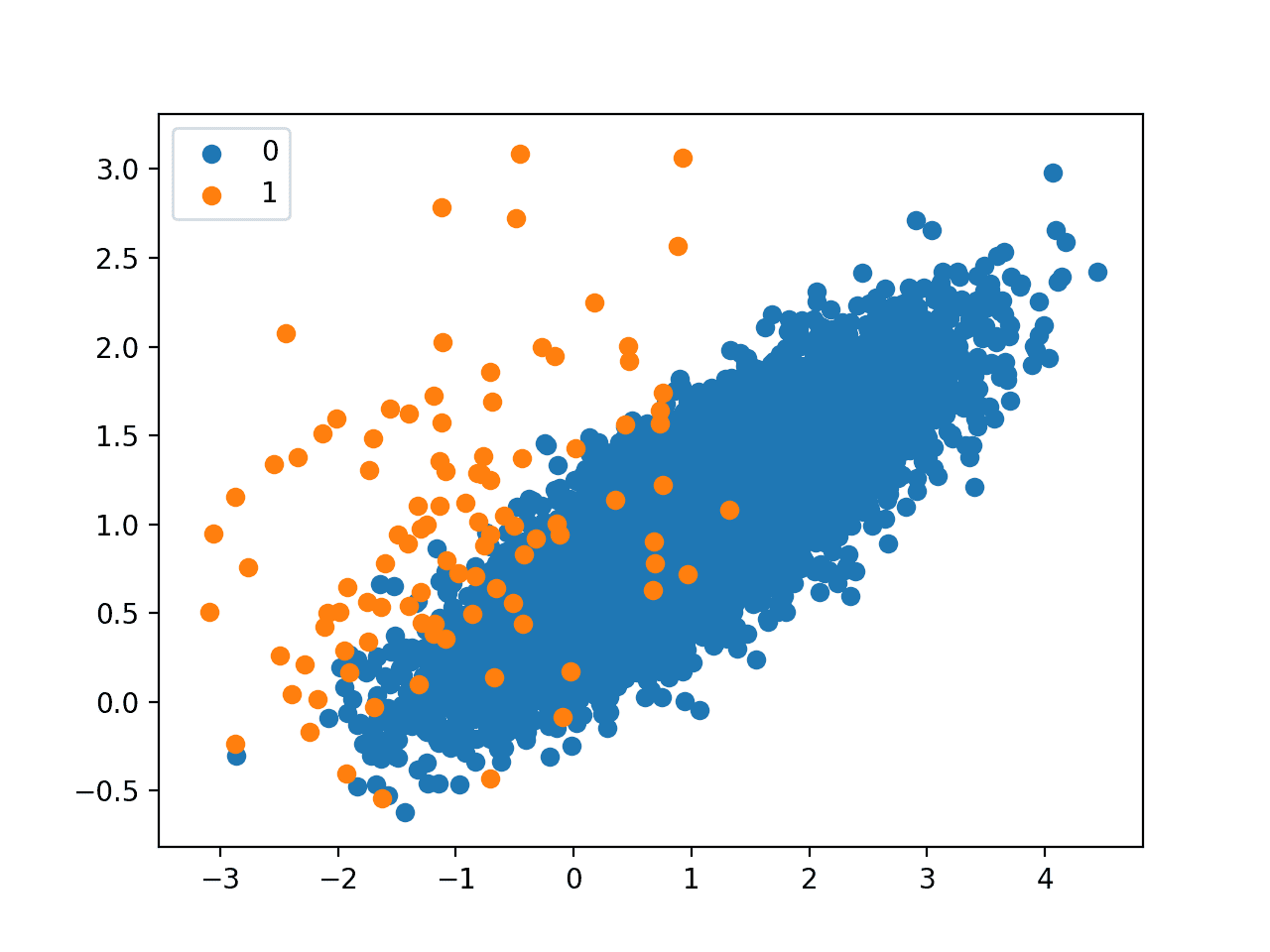
Scatter Plot of Imbalanced Classification Dataset
We can fit a DecisionTreeClassifier model on this dataset. It is a good model to test because it is sensitive to the class distribution in the training dataset.
...
# define model
model = DecisionTreeClassifier()
We can evaluate the model using repeated stratified k-fold cross-validation with three repeats and 10 folds.
The ROC area under curve (AUC) measure can be used to estimate the performance of the model. It can be optimistic for severely imbalanced datasets, although it does correctly show relative improvements in model performance.
...
# define evaluation procedure
cv = RepeatedStratifiedKFold(n_splits=10, n_repeats=3, random_state=1)
# evaluate model
scores = cross_val_score(model, X, y, scoring='roc_auc', cv=cv, n_jobs=-1)
# summarize performance
print('Mean ROC AUC: %.3f' % mean(scores))
Tying this together, the example below evaluates a decision tree model on the imbalanced classification dataset.
# evaluates a decision tree model on the imbalanced dataset
from numpy import mean
from sklearn.datasets import make_classification
from sklearn.tree import DecisionTreeClassifier
from sklearn.model_selection import cross_val_score
from sklearn.model_selection import RepeatedStratifiedKFold
# generate 2 class dataset
X, y = make_classification(n_samples=10000, n_features=2, n_redundant=0,
	n_clusters_per_class=1, weights=[0.99], flip_y=0, random_state=1)
# define model
model = DecisionTreeClassifier()
# define evaluation procedure
cv = RepeatedStratifiedKFold(n_splits=10, n_repeats=3, random_state=1)
# evaluate model
scores = cross_val_score(model, X, y, scoring='roc_auc', cv=cv, n_jobs=-1)
# summarize performance
print('Mean ROC AUC: %.3f' % mean(scores))
Running the example reports the average ROC AUC for the decision tree on the dataset over three repeats of 10-fold cross-validation (e.g. average over 30 different model evaluations).
Your specific results will vary given the stochastic nature of the learning algorithm and the evaluation procedure. Try running the example a few times.
In this example, you can see that the model achieved a ROC AUC of about 0.76. This provides a baseline on this dataset, which we can use to compare different combinations of over and under sampling methods on the training dataset.
Mean ROC AUC: 0.762
Now that we have a test problem, model, and test harness, let’s look at manual combinations of oversampling and undersampling methods.
Want to Get Started With Imbalance Classification?
Take my free 7-day email crash course now (with sample code).
Click to sign-up and also get a free PDF Ebook version of the course.
Imbalanced-Learn Library
In these examples, we will use the implementations provided by the imbalanced-learn Python library, which can be installed via pip as follows:
sudo pip install imbalanced-learn
You can confirm that the installation was successful by printing the version of the installed library:
# check version number
import imblearn
print(imblearn.__version__)
Running the example will print the version number of the installed library; for example:
0.5.0
Manually Combine Over- and Undersampling Methods
The imbalanced-learn Python library provides a range of resampling techniques, as well as a Pipeline class that can be used to create a combined sequence of resampling methods to apply to a dataset.
We can use the Pipeline to construct a sequence of oversampling and undersampling techniques to apply to a dataset. For example:
# define resampling
over = ...
under = ...
# define pipeline
pipeline = Pipeline(steps=[('o', over), ('u', under)])
This pipeline first applies an oversampling technique to a dataset, then applies undersampling to the output of the oversampling transform before returning the final outcome. It allows transforms to be stacked or applied in sequence on a dataset.
The pipeline can then be used to transform a dataset; for example:
# fit and apply the pipeline
X_resampled, y_resampled = pipeline.fit_resample(X, y)
Alternately, a model can be added as the last step in the pipeline.
This allows the pipeline to be treated as a model. When it is fit on a training dataset, the transforms are first applied to the training dataset, then the transformed dataset is provided to the model so that it can develop a fit.
...
# define model
model = ...
# define resampling
over = ...
under = ...
# define pipeline
pipeline = Pipeline(steps=[('o', over), ('u', under), ('m', model)])
Recall that the resampling is only applied to the training dataset, not the test dataset.
When used in k-fold cross-validation, the entire sequence of transforms and fit is applied on each training dataset comprised of cross-validation folds. This is important as both the transforms and fit are performed without knowledge of the holdout set, which avoids data leakage. For example:
...
# define evaluation procedure
cv = RepeatedStratifiedKFold(n_splits=10, n_repeats=3, random_state=1)
# evaluate model
scores = cross_val_score(pipeline, X, y, scoring='roc_auc', cv=cv, n_jobs=-1)
Now that we know how to manually combine resampling methods, let’s look at two examples.
Manually Combine Random Oversampling and Undersampling
A good starting point for combining resampling techniques is to start with random or naive methods.
Although they are simple, and often ineffective when applied in isolation, they can be effective when combined.
Random oversampling involves randomly duplicating examples in the minority class, whereas random undersampling involves randomly deleting examples from the majority class.
As these two transforms are performed on separate classes, the order in which they are applied to the training dataset does not matter.
The example below defines a pipeline that first oversamples the minority class to 10 percent of the majority class, under samples the majority class to 50 percent more than the minority class, and then fits a decision tree model.
...
# define model
model = DecisionTreeClassifier()
# define resampling
over = RandomOverSampler(sampling_strategy=0.1)
under = RandomUnderSampler(sampling_strategy=0.5)
# define pipeline
pipeline = Pipeline(steps=[('o', over), ('u', under), ('m', model)])
The complete example of evaluating this combination on the binary classification problem is listed below.
# combination of random oversampling and undersampling for imbalanced classification
from numpy import mean
from sklearn.datasets import make_classification
from sklearn.model_selection import cross_val_score
from sklearn.model_selection import RepeatedStratifiedKFold
from sklearn.tree import DecisionTreeClassifier
from imblearn.pipeline import Pipeline
from imblearn.over_sampling import RandomOverSampler
from imblearn.under_sampling import RandomUnderSampler
# generate dataset
X, y = make_classification(n_samples=10000, n_features=2, n_redundant=0,
	n_clusters_per_class=1, weights=[0.99], flip_y=0, random_state=1)
# define model
model = DecisionTreeClassifier()
# define resampling
over = RandomOverSampler(sampling_strategy=0.1)
under = RandomUnderSampler(sampling_strategy=0.5)
# define pipeline
pipeline = Pipeline(steps=[('o', over), ('u', under), ('m', model)])
# define evaluation procedure
cv = RepeatedStratifiedKFold(n_splits=10, n_repeats=3, random_state=1)
# evaluate model
scores = cross_val_score(pipeline, X, y, scoring='roc_auc', cv=cv, n_jobs=-1)
# summarize performance
print('Mean ROC AUC: %.3f' % mean(scores))
Running the example evaluates the system of transforms and the model and summarizes the performance as the mean ROC AUC.
Your specific results will vary given the stochastic nature of the learning algorithm, resampling algorithms, and the evaluation procedure. Try running the example a few times.
In this case, we can see a modest lift in ROC AUC performance from 0.76 with no transforms to about 0.81 with random over- and undersampling.
Mean ROC AUC: 0.814
Manually Combine SMOTE and Random Undersampling
We are not limited to using random resampling methods.
Perhaps the most popular oversampling method is the Synthetic Minority Oversampling Technique, or SMOTE for short.
SMOTE works by selecting examples that are close in the feature space, drawing a line between the examples in the feature space and drawing a new sample as a point along that line.
The authors of the technique recommend using SMOTE on the minority class, followed by an undersampling technique on the majority class.
The combination of SMOTE and under-sampling performs better than plain under-sampling.
— SMOTE: Synthetic Minority Over-sampling Technique, 2011.
We can combine SMOTE with RandomUnderSampler. Again, the order in which these procedures are applied does not matter as they are performed on different subsets of the training dataset.
The pipeline below implements this combination, first applying SMOTE to bring the minority class distribution to 10 percent of the majority class, then using RandomUnderSampler to bring the minority class down to 50 percent more than the minority class before fitting a DecisionTreeClassifier.
...
# define model
model = DecisionTreeClassifier()
# define pipeline
over = SMOTE(sampling_strategy=0.1)
under = RandomUnderSampler(sampling_strategy=0.5)
steps = [('o', over), ('u', under), ('m', model)]
The example below evaluates this combination on our imbalanced binary classification problem.
# combination of SMOTE and random undersampling for imbalanced classification
from numpy import mean
from sklearn.datasets import make_classification
from sklearn.model_selection import cross_val_score
from sklearn.model_selection import RepeatedStratifiedKFold
from sklearn.tree import DecisionTreeClassifier
from imblearn.pipeline import Pipeline
from imblearn.over_sampling import SMOTE
from imblearn.under_sampling import RandomUnderSampler
# generate dataset
X, y = make_classification(n_samples=10000, n_features=2, n_redundant=0,
	n_clusters_per_class=1, weights=[0.99], flip_y=0, random_state=1)
# define model
model = DecisionTreeClassifier()
# define pipeline
over = SMOTE(sampling_strategy=0.1)
under = RandomUnderSampler(sampling_strategy=0.5)
steps = [('o', over), ('u', under), ('m', model)]
pipeline = Pipeline(steps=steps)
# define evaluation procedure
cv = RepeatedStratifiedKFold(n_splits=10, n_repeats=3, random_state=1)
# evaluate model
scores = cross_val_score(pipeline, X, y, scoring='roc_auc', cv=cv, n_jobs=-1)
# summarize performance
print('Mean ROC AUC: %.3f' % mean(scores))
Running the example evaluates the system of transforms and the model and summarizes the performance as the mean ROC AUC.
Your specific results will vary given the stochastic nature of the learning algorithm, resampling algorithms, and the evaluation procedure. Try running the example a few times.
In this case, we can see another list in ROC AUC performance from about 0.81 to about 0.83.
Mean ROC AUC: 0.833
Use Predefined Combinations of Resampling Methods
There are combinations of oversampling and undersampling methods that have proven effective and together may be considered resampling techniques.
Two examples are the combination of SMOTE with Tomek Links undersampling and SMOTE with Edited Nearest Neighbors undersampling.
The imbalanced-learn Python library provides implementations for both of these combinations directly. Let’s take a closer look at each in turn.
Combination of SMOTE and Tomek Links Undersampling
SMOTE is an oversampling method that synthesizes new plausible examples in the majority class.
Tomek Links refers to a method for identifying pairs of nearest neighbors in a dataset that have different classes. Removing one or both of the examples in these pairs (such as the examples in the majority class) has the effect of making the decision boundary in the training dataset less noisy or ambiguous.
Gustavo Batista, et al. tested combining these methods in their 2003 paper titled “Balancing Training Data for Automated Annotation of Keywords: a Case Study.”
Specifically, first the SMOTE method is applied to oversample the minority class to a balanced distribution, then examples in Tomek Links from the majority classes are identified and removed.
In this work, only majority class examples that participate of a Tomek link were removed, since minority class examples were considered too rare to be discarded. […] In our work, as minority class examples were artificially created and the data sets are currently balanced, then both majority and minority class examples that form a Tomek link, are removed.
— Balancing Training Data for Automated Annotation of Keywords: a Case Study, 2003.
The combination was shown to provide a reduction in false negatives at the cost of an increase in false positives for a binary classification task.
We can implement this combination using the SMOTETomek class.
...
# define resampling
resample = SMOTETomek()
The SMOTE configuration can be set via the “smote” argument and takes a configured SMOTE instance. The Tomek Links configuration can be set via the “tomek” argument and takes a configured TomekLinks object.
The default is to balance the dataset with SMOTE then remove Tomek links from all classes. This is the approach used in another paper that explorea this combination titled “A Study of the Behavior of Several Methods for Balancing Machine Learning Training Data.”
… we propose applying Tomek links to the over-sampled training set as a data cleaning method. Thus, instead of removing only the majority class examples that form Tomek links, examples from both classes are removed.
— A Study of the Behavior of Several Methods for Balancing Machine Learning Training Data, 2004.
Alternately, we can configure the combination to only remove links from the majority class as described in the 2003 paper by specifying the “tomek” argument with an instance of TomekLinks with the “sampling_strategy” argument set to only undersample the ‘majority‘ class; for example:
...
# define resampling
resample = SMOTETomek(tomek=TomekLinks(sampling_strategy='majority'))
We can evaluate this combined resampling strategy with a decision tree classifier on our binary classification problem.
The complete example is listed below.
# combined SMOTE and Tomek Links resampling for imbalanced classification
from numpy import mean
from sklearn.datasets import make_classification
from sklearn.model_selection import cross_val_score
from sklearn.model_selection import RepeatedStratifiedKFold
from imblearn.pipeline import Pipeline
from sklearn.tree import DecisionTreeClassifier
from imblearn.combine import SMOTETomek
from imblearn.under_sampling import TomekLinks
# generate dataset
X, y = make_classification(n_samples=10000, n_features=2, n_redundant=0,
	n_clusters_per_class=1, weights=[0.99], flip_y=0, random_state=1)
# define model
model = DecisionTreeClassifier()
# define resampling
resample = SMOTETomek(tomek=TomekLinks(sampling_strategy='majority'))
# define pipeline
pipeline = Pipeline(steps=[('r', resample), ('m', model)])
# define evaluation procedure
cv = RepeatedStratifiedKFold(n_splits=10, n_repeats=3, random_state=1)
# evaluate model
scores = cross_val_score(pipeline, X, y, scoring='roc_auc', cv=cv, n_jobs=-1)
# summarize performance
print('Mean ROC AUC: %.3f' % mean(scores))
Running the example evaluates the system of transforms and the model and summarizes the performance as the mean ROC AUC.
Your specific results will vary given the stochastic nature of the learning algorithm, resampling algorithms, and the evaluation procedure. Try running the example a few times.
In this case, it seems that this combined resampling strategy does not offer a benefit for this model on this dataset.
Mean ROC AUC: 0.815
Combination of SMOTE and Edited Nearest Neighbors Undersampling
SMOTE may be the most popular oversampling technique and can be combined with many different undersampling techniques.
Another very popular undersampling method is the Edited Nearest Neighbors, or ENN, rule. This rule involves using k=3 nearest neighbors to locate those examples in a dataset that are misclassified and that are then removed. It can be applied to all classes or just those examples in the majority class.
Gustavo Batista, et al. explore many combinations of oversampling and undersampling methods compared to the methods used in isolation in their 2004 paper titled “A Study of the Behavior of Several Methods for Balancing Machine Learning Training Data.”
This includes the combinations:
- Condensed Nearest Neighbors + Tomek Links
- SMOTE + Tomek Links
- SMOTE + Edited NearestNeighbors
Regarding this final combination, the authors comment that ENN is more aggressive at downsampling the majority class than Tomek Links, providing more in-depth cleaning. They apply the method, removing examples from both the majority and minority classes.
… ENN is used to remove examples from both classes. Thus, any example that is misclassified by its three nearest neighbors is removed from the training set.
— A Study of the Behavior of Several Methods for Balancing Machine Learning Training Data, 2004.
This can be implemented via the SMOTEENN class in the imbalanced-learn library.
...
# define resampling
resample = SMOTEENN()
The SMOTE configuration can be set as a SMOTE object via the “smote” argument, and the ENN configuration can be set via the EditedNearestNeighbours object via the “enn” argument. SMOTE defaults to balancing the distribution, followed by ENN that by default removes misclassified examples from all classes.
We could change the ENN to only remove examples from the majority class by setting the “enn” argument to an EditedNearestNeighbours instance with sampling_strategy argument set to ‘majority‘.
...
# define resampling
resample = SMOTEENN(enn=EditedNearestNeighbours(sampling_strategy='majority'))
We can evaluate the default strategy (editing examples in all classes) and evaluate it with a decision tree classifier on our imbalanced dataset.
The complete example is listed below.
# combined SMOTE and Edited Nearest Neighbors resampling for imbalanced classification
from numpy import mean
from sklearn.datasets import make_classification
from sklearn.model_selection import cross_val_score
from sklearn.model_selection import RepeatedStratifiedKFold
from imblearn.pipeline import Pipeline
from sklearn.tree import DecisionTreeClassifier
from imblearn.combine import SMOTEENN
# generate dataset
X, y = make_classification(n_samples=10000, n_features=2, n_redundant=0,
	n_clusters_per_class=1, weights=[0.99], flip_y=0, random_state=1)
# define model
model = DecisionTreeClassifier()
# define resampling
resample = SMOTEENN()
# define pipeline
pipeline = Pipeline(steps=[('r', resample), ('m', model)])
# define evaluation procedure
cv = RepeatedStratifiedKFold(n_splits=10, n_repeats=3, random_state=1)
# evaluate model
scores = cross_val_score(pipeline, X, y, scoring='roc_auc', cv=cv, n_jobs=-1)
# summarize performance
print('Mean ROC AUC: %.3f' % mean(scores))
Running the example evaluates the system of transforms and the model and summarizes the performance as the mean ROC AUC.
Your specific results will vary given the stochastic nature of the learning algorithm, resampling algorithms, and the evaluation procedure. Try running the example a few times.
In this case, we see a further lift in performance over SMOTE with the random undersampling method from about 0.81 to about 0.85.
Mean ROC AUC: 0.856
This result highlights that editing the oversampled minority class may also be an important consideration that could easily be overlooked.
This was the same finding in the 2004 paper where the authors discover that SMOTE with Tomek Links and SMOTE with ENN perform well across a range of datasets.
Our results show that the over-sampling methods in general, and Smote + Tomek and Smote + ENN (two of the methods proposed in this work) in particular for data sets with few positive (minority) examples, provided very good results in practice.
— A Study of the Behavior of Several Methods for Balancing Machine Learning Training Data, 2004.
Further Reading
This section provides more resources on the topic if you are looking to go deeper.
Papers
- SMOTE: Synthetic Minority Over-sampling Technique, 2011.
- Balancing Training Data for Automated Annotation of Keywords: a Case Study, 2003.
- A Study of the Behavior of Several Methods for Balancing Machine Learning Training Data, 2004.
Books
- Learning from Imbalanced Data Sets, 2018.
- Imbalanced Learning: Foundations, Algorithms, and Applications, 2013.
API
- imbalanced-learn, GitHub.
- Combination of over- and under-sampling, Imbalanced Learn User Guide.
- imblearn.over_sampling.RandomOverSampler API.
- imblearn.pipeline.Pipeline API.
- imblearn.under_sampling.RandomUnderSampler API.
- imblearn.over_sampling.SMOTE API.
- imblearn.combine.SMOTETomek API.
- imblearn.combine.SMOTEENN API.
Articles
Summary
In this tutorial, you discovered how to combine oversampling and undersampling techniques for imbalanced classification.
Specifically, you learned:
- How to define a sequence of oversampling and undersampling methods to be applied to a training dataset or when evaluating a classifier model.
- How to manually combine oversampling and undersampling methods for imbalanced classification.
- How to use pre-defined and well-performing combinations of resampling methods for imbalanced classification.
Do you have any questions?
Ask your questions in the comments below and I will do my best to answer.
The post Combine Oversampling and Undersampling for Imbalanced Classification appeared first on Machine Learning Mastery.