
Author: Jason Brownlee
The decision tree algorithm is effective for balanced classification, although it does not perform well on imbalanced datasets.
The split points of the tree are chosen to best separate examples into two groups with minimum mixing. When both groups are dominated by examples from one class, the criterion used to select a split point will see good separation, when in fact, the examples from the minority class are being ignored.
This problem can be overcome by modifying the criterion used to evaluate split points to take the importance of each class into account, referred to generally as the weighted split-point or weighted decision tree.
In this tutorial, you will discover the weighted decision tree for imbalanced classification.
After completing this tutorial, you will know:
- How the standard decision tree algorithm does not support imbalanced classification.
- How the decision tree algorithm can be modified to weight model error by class weight when selecting splits.
- How to configure class weight for the decision tree algorithm and how to grid search different class weight configurations.
Discover SMOTE, one-class classification, cost-sensitive learning, threshold moving, and much more in my new book, with 30 step-by-step tutorials and full Python source code.
Let’s get started.

How to Implement Weighted Decision Trees for Imbalanced Classification
Photo by Bonnie Moreland, some rights reserved.
Tutorial Overview
This tutorial is divided into four parts; they are:
- Imbalanced Classification Dataset
- Decision Trees for Imbalanced Classification
- Weighted Decision Trees With Scikit-Learn
- Grid Search Weighted Decision Trees
Imbalanced Classification Dataset
Before we dive into the modification of decision for imbalanced classification, let’s first define an imbalanced classification dataset.
We can use the make_classification() function to define a synthetic imbalanced two-class classification dataset. We will generate 10,000 examples with an approximate 1:100 minority to majority class ratio.
...
# define dataset
X, y = make_classification(n_samples=10000, n_features=2, n_redundant=0,
	n_clusters_per_class=1, weights=[0.99], flip_y=0, random_state=3)
Once generated, we can summarize the class distribution to confirm that the dataset was created as we expected.
...
# summarize class distribution
counter = Counter(y)
print(counter)
Finally, we can create a scatter plot of the examples and color them by class label to help understand the challenge of classifying examples from this dataset.
...
# scatter plot of examples by class label
for label, _ in counter.items():
	row_ix = where(y == label)[0]
	pyplot.scatter(X[row_ix, 0], X[row_ix, 1], label=str(label))
pyplot.legend()
pyplot.show()
Tying this together, the complete example of generating the synthetic dataset and plotting the examples is listed below.
# Generate and plot a synthetic imbalanced classification dataset
from collections import Counter
from sklearn.datasets import make_classification
from matplotlib import pyplot
from numpy import where
# define dataset
X, y = make_classification(n_samples=10000, n_features=2, n_redundant=0,
	n_clusters_per_class=1, weights=[0.99], flip_y=0, random_state=3)
# summarize class distribution
counter = Counter(y)
print(counter)
# scatter plot of examples by class label
for label, _ in counter.items():
	row_ix = where(y == label)[0]
	pyplot.scatter(X[row_ix, 0], X[row_ix, 1], label=str(label))
pyplot.legend()
pyplot.show()
Running the example first creates the dataset and summarizes the class distribution.
We can see that the dataset has an approximate 1:100 class distribution with a little less than 10,000 examples in the majority class and 100 in the minority class.
Counter({0: 9900, 1: 100})
Next, a scatter plot of the dataset is created showing the large mass of examples for the majority class (blue) and a small number of examples for the minority class (orange), with some modest class overlap.
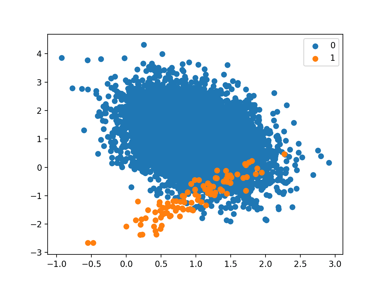
Scatter Plot of Binary Classification Dataset With 1 to 100 Class Imbalance
Next, we can fit a standard decision tree model on the dataset.
A decision tree can be defined using the DecisionTreeClassifier class in the scikit-learn library.
...
# define model
model = DecisionTreeClassifier()
We will use repeated cross-validation to evaluate the model, with three repeats of 10-fold cross-validation. The mode performance will be reported using the mean ROC area under curve (ROC AUC) averaged over repeats and all folds.
...
# define evaluation procedure
cv = RepeatedStratifiedKFold(n_splits=10, n_repeats=3, random_state=1)
# evaluate model
scores = cross_val_score(model, X, y, scoring='roc_auc', cv=cv, n_jobs=-1)
# summarize performance
print('Mean ROC AUC: %.3f' % mean(scores))
Tying this together, the complete example of defining and evaluating a standard decision tree model on the imbalanced classification problem is listed below.
Decision trees are an effective model for binary classification tasks, although by default, they are not effective at imbalanced classification.
# fit a decision tree on an imbalanced classification dataset
from numpy import mean
from sklearn.datasets import make_classification
from sklearn.model_selection import cross_val_score
from sklearn.model_selection import RepeatedStratifiedKFold
from sklearn.tree import DecisionTreeClassifier
# generate dataset
X, y = make_classification(n_samples=10000, n_features=2, n_redundant=0,
	n_clusters_per_class=1, weights=[0.99], flip_y=0, random_state=3)
# define model
model = DecisionTreeClassifier()
# define evaluation procedure
cv = RepeatedStratifiedKFold(n_splits=10, n_repeats=3, random_state=1)
# evaluate model
scores = cross_val_score(model, X, y, scoring='roc_auc', cv=cv, n_jobs=-1)
# summarize performance
print('Mean ROC AUC: %.3f' % mean(scores))
Running the example evaluates the standard decision tree model on the imbalanced dataset and reports the mean ROC AUC.
Your specific results may vary given the stochastic nature of the learning algorithm. Try running the example a few times.
We can see that the model has skill, achieving a ROC AUC above 0.5, in this case achieving a mean score of 0.746.
Mean ROC AUC: 0.746
This provides a baseline for comparison for any modifications performed to the standard decision tree algorithm.
Want to Get Started With Imbalance Classification?
Take my free 7-day email crash course now (with sample code).
Click to sign-up and also get a free PDF Ebook version of the course.
Decision Trees for Imbalanced Classification
The decision tree algorithm is also known as Classification and Regression Trees (CART) and involves growing a tree to classify examples from the training dataset.
The tree can be thought to divide the training dataset, where examples progress down the decision points of the tree to arrive in the leaves of the tree and are assigned a class label.
The tree is constructed by splitting the training dataset using values for variables in the dataset. At each point, the split in the data that results in the purest (least mixed) groups of examples is chosen in a greedy manner.
Here, purity means a clean separation of examples into groups where a group of examples of all 0 or all 1 class is the purest, and a 50-50 mixture of both classes is the least pure. Purity is most commonly calculated using Gini impurity, although it can also be calculated using entropy.
The calculation of a purity measure involves calculating the probability of an example of a given class being misclassified by a split. Calculating these probabilities involves summing the number of examples in each class within each group.
The splitting criterion can be updated to not only take the purity of the split into account, but also be weighted by the importance of each class.
Our intuition for cost-sensitive tree induction is to modify the weight of an instance proportional to the cost of misclassifying the class to which the instance belonged …
—An Instance-weighting Method To Induce Cost-sensitive Trees, 2002.
This can be achieved by replacing the count of examples in each group by a weighted sum, where the coefficient is provided to weight the sum.
Larger weight is assigned to the class with more importance, and a smaller weight is assigned to a class with less importance.
- Small Weight: Less importance, lower impact on node purity.
- Large Weight: More importance, higher impact on node purity.
A small weight can be assigned to the majority class, which has the effect of improving (lowering) the purity score of a node that may otherwise look less well sorted. In turn, this may allow more examples from the majority class to be classified for the minority class, better accommodating those examples in the minority class.
Higher weights [are] assigned to instances coming from the class with a higher value of misclassification cost.
— Page 71, Learning from Imbalanced Data Sets, 2018.
As such, this modification of the decision tree algorithm is referred to as a weighted decision tree, a class-weighted decision tree, or a cost-sensitive decision tree.
Modification of the split point calculation is the most common, although there has been a lot of research into a range of other modifications of the decision tree construction algorithm to better accommodate a class imbalance.
Weighted Decision Tree With Scikit-Learn
The scikit-learn Python machine learning library provides an implementation of the decision tree algorithm that supports class weighting.
The DecisionTreeClassifier class provides the class_weight argument that can be specified as a model hyperparameter. The class_weight is a dictionary that defines each class label (e.g. 0 and 1) and the weighting to apply in the calculation of group purity for splits in the decision tree when fitting the model.
For example, a 1 to 1 weighting for each class 0 and 1 can be defined as follows:
...
# define model
weights = {0:1.0, 1:1.0}
model = DecisionTreeClassifier(class_weight=weights)
The class weighing can be defined multiple ways; for example:
- Domain expertise, determined by talking to subject matter experts.
- Tuning, determined by a hyperparameter search such as a grid search.
- Heuristic, specified using a general best practice.
A best practice for using the class weighting is to use the inverse of the class distribution present in the training dataset.
For example, the class distribution of the test dataset is a 1:100 ratio for the minority class to the majority class. The invert of this ratio could be used with 1 for the majority class and 100 for the minority class.
For example:
...
# define model
weights = {0:1.0, 1:100.0}
model = DecisionTreeClassifier(class_weight=weights)
We might also define the same ratio using fractions and achieve the same result.
For example:
...
# define model
weights = {0:0.01, 1:1.0}
model = DecisionTreeClassifier(class_weight=weights)
This heuristic is available directly by setting the class_weight to ‘balanced.’
For example:
...
# define model
model = DecisionTreeClassifier(class_weight='balanced')
We can evaluate the decision tree algorithm with a class weighting using the same evaluation procedure defined in the previous section.
We would expect the class-weighted version of the decision tree to perform better than the standard version of the decision tree without any class weighting.
The complete example is listed below.
# decision tree with class weight on an imbalanced classification dataset
from numpy import mean
from sklearn.datasets import make_classification
from sklearn.model_selection import cross_val_score
from sklearn.model_selection import RepeatedStratifiedKFold
from sklearn.tree import DecisionTreeClassifier
# generate dataset
X, y = make_classification(n_samples=10000, n_features=2, n_redundant=0,
	n_clusters_per_class=1, weights=[0.99], flip_y=0, random_state=3)
# define model
model = DecisionTreeClassifier(class_weight='balanced')
# define evaluation procedure
cv = RepeatedStratifiedKFold(n_splits=10, n_repeats=3, random_state=1)
# evaluate model
scores = cross_val_score(model, X, y, scoring='roc_auc', cv=cv, n_jobs=-1)
# summarize performance
print('Mean ROC AUC: %.3f' % mean(scores))
Running the example prepares the synthetic imbalanced classification dataset, then evaluates the class-weighted version of the decision tree algorithm using repeated cross-validation.
Your specific results may vary given the stochastic nature of the learning algorithm. Try running the example a few times.
The mean ROC AUC score is reported, in this case, showing a better score than the unweighted version of the decision tree algorithm: 0.759 as compared to 0.746.
Mean ROC AUC: 0.759
Grid Search Weighted Decision Tree
Using a class weighting that is the inverse ratio of the training data is just a heuristic.
It is possible that better performance can be achieved with a different class weighting, and this too will depend on the choice of performance metric used to evaluate the model.
In this section, we will grid search a range of different class weightings for the weighted decision tree and discover which results in the best ROC AUC score.
We will try the following weightings for class 0 and 1:
- Class 0:100, Class 1:1.
- Class 0:10, Class 1:1.
- Class 0:1, Class 1:1.
- Class 0:1, Class 1:10.
- Class 0:1, Class 1:100.
These can be defined as grid search parameters for the GridSearchCV class as follows:
...
# define grid
balance = [{0:100,1:1}, {0:10,1:1}, {0:1,1:1}, {0:1,1:10}, {0:1,1:100}]
param_grid = dict(class_weight=balance)
We can perform the grid search on these parameters using repeated cross-validation and estimate model performance using ROC AUC:
...
# define evaluation procedure
cv = RepeatedStratifiedKFold(n_splits=10, n_repeats=3, random_state=1)
# define grid search
grid = GridSearchCV(estimator=model, param_grid=param_grid, n_jobs=-1, cv=cv, scoring='roc_auc')
Once executed, we can summarize the best configuration as well as all of the results as follows:
...
# report the best configuration
print("Best: %f using %s" % (grid_result.best_score_, grid_result.best_params_))
# report all configurations
means = grid_result.cv_results_['mean_test_score']
stds = grid_result.cv_results_['std_test_score']
params = grid_result.cv_results_['params']
for mean, stdev, param in zip(means, stds, params):
    print("%f (%f) with: %r" % (mean, stdev, param))
Tying this together, the example below grid searches five different class weights for the decision tree algorithm on the imbalanced dataset.
We might expect that the heuristic class weighing is the best performing configuration.
# grid search class weights with decision tree for imbalance classification
from numpy import mean
from sklearn.datasets import make_classification
from sklearn.model_selection import GridSearchCV
from sklearn.model_selection import RepeatedStratifiedKFold
from sklearn.tree import DecisionTreeClassifier
# generate dataset
X, y = make_classification(n_samples=10000, n_features=2, n_redundant=0,
	n_clusters_per_class=1, weights=[0.99], flip_y=0, random_state=3)
# define model
model = DecisionTreeClassifier()
# define grid
balance = [{0:100,1:1}, {0:10,1:1}, {0:1,1:1}, {0:1,1:10}, {0:1,1:100}]
param_grid = dict(class_weight=balance)
# define evaluation procedure
cv = RepeatedStratifiedKFold(n_splits=10, n_repeats=3, random_state=1)
# define grid search
grid = GridSearchCV(estimator=model, param_grid=param_grid, n_jobs=-1, cv=cv, scoring='roc_auc')
# execute the grid search
grid_result = grid.fit(X, y)
# report the best configuration
print("Best: %f using %s" % (grid_result.best_score_, grid_result.best_params_))
# report all configurations
means = grid_result.cv_results_['mean_test_score']
stds = grid_result.cv_results_['std_test_score']
params = grid_result.cv_results_['params']
for mean, stdev, param in zip(means, stds, params):
    print("%f (%f) with: %r" % (mean, stdev, param))
Running the example evaluates each class weighting using repeated k-fold cross-validation and reports the best configuration and the associated mean ROC AUC score.
Your specific results may vary given the stochastic nature of the learning algorithm. Try running the example a few times.
In this case, we can see that the 1:100 majority to minority class weighting achieved the best mean ROC score. This matches the configuration for the general heuristic.
It might be interesting to explore even more severe class weightings to see their effect on the mean ROC AUC score.
Best: 0.752643 using {'class_weight': {0: 1, 1: 100}}
0.737306 (0.080007) with: {'class_weight': {0: 100, 1: 1}}
0.747306 (0.075298) with: {'class_weight': {0: 10, 1: 1}}
0.740606 (0.074948) with: {'class_weight': {0: 1, 1: 1}}
0.747407 (0.068104) with: {'class_weight': {0: 1, 1: 10}}
0.752643 (0.073195) with: {'class_weight': {0: 1, 1: 100}}
Further Reading
This section provides more resources on the topic if you are looking to go deeper.
Papers
Books
- Learning from Imbalanced Data Sets, 2018.
- Imbalanced Learning: Foundations, Algorithms, and Applications, 2013.
APIs
- sklearn.utils.class_weight.compute_class_weight API.
- sklearn.tree.DecisionTreeClassifier API.
- sklearn.model_selection.GridSearchCV API.
Summary
In this tutorial, you discovered the weighted decision tree for imbalanced classification.
Specifically, you learned:
- How the standard decision tree algorithm does not support imbalanced classification.
- How the decision tree algorithm can be modified to weight model error by class weight when selecting splits.
- How to configure class weight for the decision tree algorithm and how to grid search different class weight configurations.
Do you have any questions?
Ask your questions in the comments below and I will do my best to answer.
The post Cost-Sensitive Decision Trees for Imbalanced Classification appeared first on Machine Learning Mastery.