Cost-Sensitive SVM for Imbalanced Classification

Author: Jason Brownlee

The Support Vector Machine algorithm is effective for balanced classification, although it does not perform well on imbalanced datasets.

The SVM algorithm finds a hyperplane decision boundary that best splits the examples into two classes. The split is made soft through the use of a margin that allows some points to be misclassified. By default, this margin favors the majority class on imbalanced datasets, although it can be updated to take the importance of each class into account and dramatically improve the performance of the algorithm on datasets with skewed class distributions.

This modification of SVM that weighs the margin proportional to the class importance is often referred to as weighted SVM, or cost-sensitive SVM.

In this tutorial, you will discover weighted support vector machines for imbalanced classification.

After completing this tutorial, you will know:

How the standard support vector machine algorithm is limited for imbalanced classification.
How the support vector machine algorithm can be modified to weight the margin penalty proportional to class importance during training.
How to configure class weight for the SVM and how to grid search different class weight configurations.

Discover SMOTE, one-class classification, cost-sensitive learning, threshold moving, and much more in my new book, with 30 step-by-step tutorials and full Python source code.

Let’s get started.

How to Implement Weighted Support Vector Machines for Imbalanced Classification
Photo by Bas Leenders, some rights reserved.

Tutorial Overview

This tutorial is divided into four parts; they are:

Imbalanced Classification Dataset
SVM for Imbalanced Classification
Weighted SVM With Scikit-Learn
Grid Search Weighted SVM

Imbalanced Classification Dataset

Before we dive into the modification of SVM for imbalanced classification, let’s first define an imbalanced classification dataset.

We can use the make_classification() function to define a synthetic imbalanced two-class classification dataset. We will generate 10,000 examples with an approximate 1:100 minority to majority class ratio.

...
# define dataset
X, y = make_classification(n_samples=10000, n_features=2, n_redundant=0,
	n_clusters_per_class=1, weights=[0.99], flip_y=0, random_state=4)

Once generated, we can summarize the class distribution to confirm that the dataset was created as we expected.

...
# summarize class distribution
counter = Counter(y)
print(counter)

Finally, we can create a scatter plot of the examples and color them by class label to help understand the challenge of classifying examples from this dataset.

...
# scatter plot of examples by class label
for label, _ in counter.items():
	row_ix = where(y == label)[0]
	pyplot.scatter(X[row_ix, 0], X[row_ix, 1], label=str(label))
pyplot.legend()
pyplot.show()

Tying this together, the complete example of generating the synthetic dataset and plotting the examples is listed below.

# Generate and plot a synthetic imbalanced classification dataset
from collections import Counter
from sklearn.datasets import make_classification
from matplotlib import pyplot
from numpy import where
# define dataset
X, y = make_classification(n_samples=10000, n_features=2, n_redundant=0,
	n_clusters_per_class=1, weights=[0.99], flip_y=0, random_state=4)
# summarize class distribution
counter = Counter(y)
print(counter)
# scatter plot of examples by class label
for label, _ in counter.items():
	row_ix = where(y == label)[0]
	pyplot.scatter(X[row_ix, 0], X[row_ix, 1], label=str(label))
pyplot.legend()
pyplot.show()

Running the example first creates the dataset and summarizes the class distribution.

We can see that the dataset has an approximate 1:100 class distribution with a little less than 10,000 examples in the majority class and 100 in the minority class.

Counter({0: 9900, 1: 100})

Next, a scatter plot of the dataset is created showing the large mass of examples for the majority class (blue) and a small number of examples for the minority class (orange), with some modest class overlap.

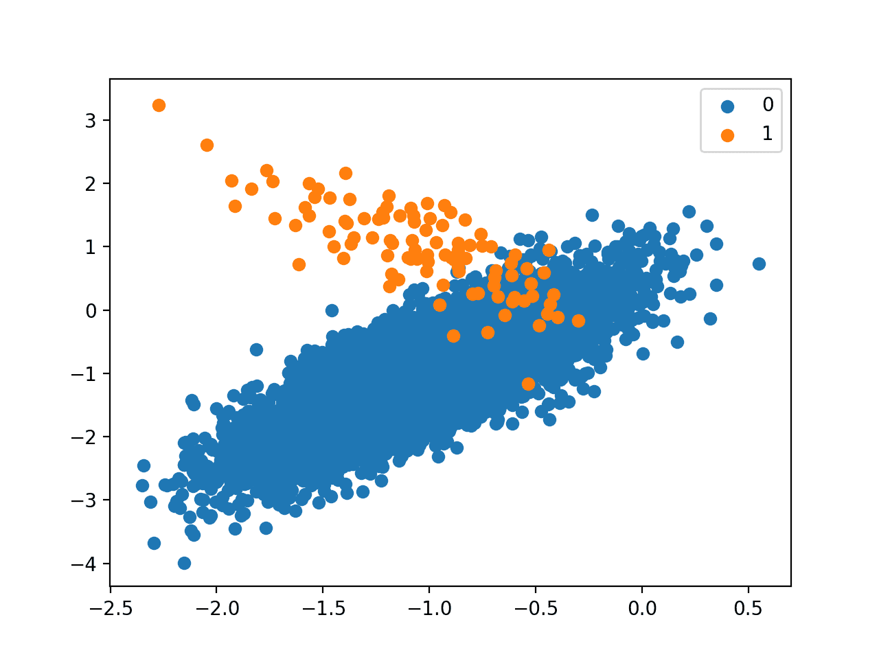
Scatter Plot of Binary Classification Dataset With 1 to 100 Class Imbalance

Next, we can fit a standard SVM model on the dataset.

An SVM can be defined using the SVC class in the scikit-learn library.

...
# define model
model = SVC(gamma='scale')

We will use repeated cross-validation to evaluate the model, with three repeats of 10-fold cross-validation. The mode performance will be reported using the mean ROC area under curve (ROC AUC) averaged over repeats and all folds.

...
# define evaluation procedure
cv = RepeatedStratifiedKFold(n_splits=10, n_repeats=3, random_state=1)
# evaluate model
scores = cross_val_score(model, X, y, scoring='roc_auc', cv=cv, n_jobs=-1)
# summarize performance
print('Mean ROC AUC: %.3f' % mean(scores))

Tying this together, the complete example of defining and evaluating a standard SVM model on the imbalanced classification problem is listed below.

SVMs are effective models for binary classification tasks, although by default, they are not effective at imbalanced classification.

# fit a svm on an imbalanced classification dataset
from numpy import mean
from sklearn.datasets import make_classification
from sklearn.model_selection import cross_val_score
from sklearn.model_selection import RepeatedStratifiedKFold
from sklearn.svm import SVC
# generate dataset
X, y = make_classification(n_samples=10000, n_features=2, n_redundant=0,
	n_clusters_per_class=1, weights=[0.99], flip_y=0, random_state=4)
# define model
model = SVC(gamma='scale')
# define evaluation procedure
cv = RepeatedStratifiedKFold(n_splits=10, n_repeats=3, random_state=1)
# evaluate model
scores = cross_val_score(model, X, y, scoring='roc_auc', cv=cv, n_jobs=-1)
# summarize performance
print('Mean ROC AUC: %.3f' % mean(scores))

Running the example evaluates the standard SVM model on the imbalanced dataset and reports the mean ROC AUC.

Your specific results may vary given the stochastic nature of the learning algorithm. Try running the example a few times.

We can see that the model has skill, achieving a ROC AUC above 0.5, in this case achieving a mean score of 0.804.

Mean ROC AUC: 0.804

This provides a baseline for comparison for any modifications performed to the standard SVM algorithm.

Want to Get Started With Imbalance Classification?

Take my free 7-day email crash course now (with sample code).

Click to sign-up and also get a free PDF Ebook version of the course.

Download Your FREE Mini-Course

SVM for Imbalanced Classification

Support Vector Machines, or SVMs for short, are an effective nonlinear machine learning algorithm.

The SVM training algorithm seeks a line or hyperplane that best separates the classes. The hyperplane is defined by a margin that maximizes the distance between the decision boundary and the closest examples from each of the two classes.

Loosely speaking, the margin is the distance between the classification boundary and the closest training set point.

— Pages 343-344, Applied Predictive Modeling, 2013.

The data may be transformed using a kernel to allow linear hyperplanes to be defined to separate the classes in a transformed feature space that corresponds to a nonlinear class boundary in the original feature space. Common kernel transforms include a linear, polynomial, and radial basis function transform. This transformation of data is referred to as the “kernel trick.”

Typically, the classes are not separable, even with data transforms. As such, the margin is softened to allow some points to appear on the wrong side of the decision boundary. This softening of the margin is controlled by a regularization hyperparameter referred to as the soft-margin parameter, lambda, or capital-C (“C“).

… where C stands for the regularization parameter that controls the trade-off between maximizing the separation margin between classes and minimizing the number of misclassified instances.

— Page 125, Learning from Imbalanced Data Sets, 2018.

A value of C indicates a hard margin and no tolerance for violations of the margin. Small positive values allow some violation, whereas large integer values, such as 1, 10, and 100 allow for a much softer margin.

… [C] determines the number and severity of the violations to the margin (and to the hyperplane) that we will tolerate. We can think of C as a budget for the amount that the margin can be violated by the n observations.

— Page 347, An Introduction to Statistical Learning: with Applications in R, 2013.

Although effective, SVMs perform poorly when there is a severe skew in the class distribution. As such, there are many extensions to the algorithm in order to make them more effective on imbalanced datasets.

Although SVMs often produce effective solutions for balanced datasets, they are sensitive to the imbalance in the datasets and produce suboptimal models.

— Page 86, Imbalanced Learning: Foundations, Algorithms, and Applications, 2013.

The C parameter is used as a penalty during the fit of the model, specifically the finding of the decision boundary. By default, each class has the same weighting, which means that the softness of the margin is symmetrical.

Given that there are significantly more examples in the majority class than the minority class, it means that the soft margin and, in turn, the decision boundary will favor the majority class.

… [the] learning algorithm will favor the majority class, as concentrating on it will lead to a better trade-off between classification error and margin maximization. This will come at the expense of minority class, especially when the imbalance ratio is high, as then ignoring the minority class will lead to better optimization results.

— Page 126, Learning from Imbalanced Data Sets, 2018.

Perhaps the simplest and most common extension to SVM for imbalanced classification is to weight the C value in proportion to the importance of each class.

To accommodate these factors in SVMs an instance-level weighted modification was proposed. […] Values of weights may be given depending on the imbalance ratio between classes or individual instance complexity factors.

— Page 130, Learning from Imbalanced Data Sets, 2018.

Specifically, each example in the training dataset has its own penalty term (C value) used in the calculation for the margin when fitting the SVM model. The value of an example’s C-value can be calculated as a weighting of the global C-value, where the weight is defined proportional to the class distribution.

C_i = weight_i * C

A larger weighting can be used for the minority class, allowing the margin to be softer, whereas a smaller weighting can be used for the majority class, forcing the margin to be harder and preventing misclassified examples.

Small Weight: Smaller C value, larger penalty for misclassified examples.
Larger Weight: Larger C value, smaller penalty for misclassified examples.

This has the effect of encouraging the margin to contain the majority class with less flexibility, but allow the minority class to be flexible with misclassification of majority class examples onto the minority class side if needed.

That is, the modified SVM algorithm would not tend to skew the separating hyperplane toward the minority class examples to reduce the total misclassifications, as the minority class examples are now assigned with a higher misclassification cost.

— Page 89, Imbalanced Learning: Foundations, Algorithms, and Applications, 2013.

This modification of SVM may be referred to as Weighted Support Vector Machine (SVM), or more generally, Class-Weighted SVM, Instance-Weighted SVM, or Cost-Sensitive SVM.

The basic idea is to assign different weights to different data points such that the WSVM training algorithm learns the decision surface according to the relative importance of data points in the training data set.

— A Weighted Support Vector Machine For Data Classification, 2007.

Weighted SVM With Scikit-Learn

The scikit-learn Python machine learning library provides an implementation of the SVM algorithm that supports class weighting.

The LinearSVC and SVC classes provide the class_weight argument that can be specified as a model hyperparameter. The class_weight is a dictionary that defines each class label (e.g. 0 and 1) and the weighting to apply to the C value in the calculation of the soft margin.

For example, a 1 to 1 weighting for each class 0 and 1 can be defined as follows:

...
# define model
weights = {0:1.0, 1:1.0}
model = SVC(gamma='scale', class_weight=weights)

The class weighing can be defined multiple ways; for example:

Domain expertise, determined by talking to subject matter experts.
Tuning, determined by a hyperparameter search such as a grid search.
Heuristic, specified using a general best practice.

A best practice for using the class weighting is to use the inverse of the class distribution present in the training dataset.

For example, the class distribution of the test dataset is a 1:100 ratio for the minority class to the majority class. The invert of this ratio could be used with 1 for the majority class and 100 for the minority class; for example:

...
# define model
weights = {0:1.0, 1:100.0}
model = SVC(gamma='scale', class_weight=weights)

We might also define the same ratio using fractions and achieve the same result; for example:

...
# define model
weights = {0:0.01, 1:1.0}
model = SVC(gamma='scale', class_weight=weights)

This heuristic is available directly by setting the class_weight to ‘balanced.’ For example:

...
# define model
model = SVC(gamma='scale', class_weight='balanced')

We can evaluate the SVM algorithm with a class weighting using the same evaluation procedure defined in the previous section.

We would expect the class-weighted version of SVM to perform better than the standard version of the SVM without any class weighting.

The complete example is listed below.

# svm with class weight on an imbalanced classification dataset
from numpy import mean
from sklearn.datasets import make_classification
from sklearn.model_selection import cross_val_score
from sklearn.model_selection import RepeatedStratifiedKFold
from sklearn.svm import SVC
# generate dataset
X, y = make_classification(n_samples=10000, n_features=2, n_redundant=0,
	n_clusters_per_class=1, weights=[0.99], flip_y=0, random_state=4)
# define model
model = SVC(gamma='scale', class_weight='balanced')
# define evaluation procedure
cv = RepeatedStratifiedKFold(n_splits=10, n_repeats=3, random_state=1)
# evaluate model
scores = cross_val_score(model, X, y, scoring='roc_auc', cv=cv, n_jobs=-1)
# summarize performance
print('Mean ROC AUC: %.3f' % mean(scores))

Running the example prepares the synthetic imbalanced classification dataset, then evaluates the class-weighted version of the SVM algorithm using repeated cross-validation.

Your specific results may vary given the stochastic nature of the learning algorithm. Try running the example a few times.

The mean ROC AUC score is reported, in this case, showing a better score than the unweighted version of the SVM algorithm, 0.964 as compared to 0.804.

Mean ROC AUC: 0.964

Grid Search Weighted SVM

Using a class weighting that is the inverse ratio of the training data is just a heuristic.

It is possible that better performance can be achieved with a different class weighting, and this too will depend on the choice of performance metric used to evaluate the model.

In this section, we will grid search a range of different class weightings for weighted SVM and discover which results in the best ROC AUC score.

We will try the following weightings for class 0 and 1:

Class 0: 100, Class 1: 1
Class 0: 10, Class 1: 1
Class 0: 1, Class 1: 1
Class 0: 1, Class 1: 10
Class 0: 1, Class 1: 100

These can be defined as grid search parameters for the GridSearchCV class as follows:

...
# define grid
balance = [{0:100,1:1}, {0:10,1:1}, {0:1,1:1}, {0:1,1:10}, {0:1,1:100}]
param_grid = dict(class_weight=balance)

We can perform the grid search on these parameters using repeated cross-validation and estimate model performance using ROC AUC:

...
# define evaluation procedure
cv = RepeatedStratifiedKFold(n_splits=10, n_repeats=3, random_state=1)
# define grid search
grid = GridSearchCV(estimator=model, param_grid=param_grid, n_jobs=-1, cv=cv, scoring='roc_auc')

Once executed, we can summarize the best configuration as well as all of the results as follows:

...
# report the best configuration
print("Best: %f using %s" % (grid_result.best_score_, grid_result.best_params_))
# report all configurations
means = grid_result.cv_results_['mean_test_score']
stds = grid_result.cv_results_['std_test_score']
params = grid_result.cv_results_['params']
for mean, stdev, param in zip(means, stds, params):
    print("%f (%f) with: %r" % (mean, stdev, param))

Tying this together, the example below grid searches five different class weights for the SVM algorithm on the imbalanced dataset.

We might expect that the heuristic class weighing is the best performing configuration.

# grid search class weights with svm for imbalance classification
from numpy import mean
from sklearn.datasets import make_classification
from sklearn.model_selection import GridSearchCV
from sklearn.model_selection import RepeatedStratifiedKFold
from sklearn.svm import SVC
# generate dataset
X, y = make_classification(n_samples=10000, n_features=2, n_redundant=0,
	n_clusters_per_class=1, weights=[0.99], flip_y=0, random_state=4)
# define model
model = SVC(gamma='scale')
# define grid
balance = [{0:100,1:1}, {0:10,1:1}, {0:1,1:1}, {0:1,1:10}, {0:1,1:100}]
param_grid = dict(class_weight=balance)
# define evaluation procedure
cv = RepeatedStratifiedKFold(n_splits=10, n_repeats=3, random_state=1)
# define grid search
grid = GridSearchCV(estimator=model, param_grid=param_grid, n_jobs=-1, cv=cv, scoring='roc_auc')
# execute the grid search
grid_result = grid.fit(X, y)
# report the best configuration
print("Best: %f using %s" % (grid_result.best_score_, grid_result.best_params_))
# report all configurations
means = grid_result.cv_results_['mean_test_score']
stds = grid_result.cv_results_['std_test_score']
params = grid_result.cv_results_['params']
for mean, stdev, param in zip(means, stds, params):
    print("%f (%f) with: %r" % (mean, stdev, param))

Running the example evaluates each class weighting using repeated k-fold cross-validation and reports the best configuration and the associated mean ROC AUC score.

Your specific results may vary given the stochastic nature of the learning algorithm. Try running the example a few times.

In this case, we can see that the 1:100 majority to minority class weighting achieved the best mean ROC score. This matches the configuration for the general heuristic.

It might be interesting to explore even more severe class weightings to see their effect on the mean ROC AUC score.

Best: 0.966189 using {'class_weight': {0: 1, 1: 100}}
0.745249 (0.129002) with: {'class_weight': {0: 100, 1: 1}}
0.748407 (0.128049) with: {'class_weight': {0: 10, 1: 1}}
0.803727 (0.103536) with: {'class_weight': {0: 1, 1: 1}}
0.932620 (0.059869) with: {'class_weight': {0: 1, 1: 10}}
0.966189 (0.036310) with: {'class_weight': {0: 1, 1: 100}}

Summary

In this tutorial, you discovered weighted support vector machines for imbalanced classification.

Specifically, you learned:

How the standard support vector machine algorithm is limited for imbalanced classification.
How the support vector machine algorithm can be modified to weight the margin penalty proportional to class importance during training.
How to configure class weight for the SVM and how to grid search different class weight configurations.

Do you have any questions?
Ask your questions in the comments below and I will do my best to answer.

The post Cost-Sensitive SVM for Imbalanced Classification appeared first on Machine Learning Mastery.

Go to Source

Cost-Sensitive SVM for Imbalanced Classification

Tutorial Overview

Imbalanced Classification Dataset

Want to Get Started With Imbalance Classification?

SVM for Imbalanced Classification

Weighted SVM With Scikit-Learn

Grid Search Weighted SVM

Further Reading

Papers

Books

Articles

Summary