
Author: Jason Brownlee
Deep learning neural networks are a flexible class of machine learning algorithms that perform well on a wide range of problems.
Neural networks are trained using the backpropagation of error algorithm that involves calculating errors made by the model on the training dataset and updating the model weights in proportion to those errors. The limitation of this method of training is that examples from each class are treated the same, which for imbalanced datasets means that the model is adapted a lot more for one class than another.
The backpropagation algorithm can be updated to weigh misclassification errors in proportion to the importance of the class, referred to as weighted neural networks or cost-sensitive neural networks. This has the effect of allowing the model to pay more attention to examples from the minority class than the majority class in datasets with a severely skewed class distribution.
In this tutorial, you will discover weighted neural networks for imbalanced classification.
After completing this tutorial, you will know:
- How the standard neural network algorithm does not support imbalanced classification.
- How the neural network training algorithm can be modified to weight misclassification errors in proportion to class importance.
- How to configure class weight for neural networks and evaluate the effect on model performance.
Discover SMOTE, one-class classification, cost-sensitive learning, threshold moving, and much more in my new book, with 30 step-by-step tutorials and full Python source code.
Let’s get started.

How to Develop a Cost-Sensitive Neural Network for Imbalanced Classification
Photo by Bernard Spragg. NZ, some rights reserved.
Tutorial Overview
This tutorial is divided into four parts; they are:
- Imbalanced Classification Dataset
- Neural Network Model in Keras
- Deep Learning for Imbalanced Classification
- Weighted Neural Network With Keras
Imbalanced Classification Dataset
Before we dive into the modification of neural networks for imbalanced classification, let’s first define an imbalanced classification dataset.
We can use the make_classification() function to define a synthetic imbalanced two-class classification dataset. We will generate 10,000 examples with an approximate 1:100 minority to majority class ratio.
...
# define dataset
X, y = make_classification(n_samples=10000, n_features=2, n_redundant=0,
	n_clusters_per_class=2, weights=[0.99], flip_y=0, random_state=4)
Once generated, we can summarize the class distribution to confirm that the dataset was created as we expected.
...
# summarize class distribution
counter = Counter(y)
print(counter)
Finally, we can create a scatter plot of the examples and color them by class label to help understand the challenge of classifying examples from this dataset.
...
# scatter plot of examples by class label
for label, _ in counter.items():
	row_ix = where(y == label)[0]
	pyplot.scatter(X[row_ix, 0], X[row_ix, 1], label=str(label))
pyplot.legend()
pyplot.show()
Tying this together, the complete example of generating the synthetic dataset and plotting the examples is listed below.
# Generate and plot a synthetic imbalanced classification dataset
from collections import Counter
from sklearn.datasets import make_classification
from matplotlib import pyplot
from numpy import where
# define dataset
X, y = make_classification(n_samples=10000, n_features=2, n_redundant=0,
	n_clusters_per_class=2, weights=[0.99], flip_y=0, random_state=4)
# summarize class distribution
counter = Counter(y)
print(counter)
# scatter plot of examples by class label
for label, _ in counter.items():
	row_ix = where(y == label)[0]
	pyplot.scatter(X[row_ix, 0], X[row_ix, 1], label=str(label))
pyplot.legend()
pyplot.show()
Running the example first creates the dataset and summarizes the class distribution.
We can see that the dataset has an approximate 1:100 class distribution with a little less than 10,000 examples in the majority class and 100 in the minority class.
Counter({0: 9900, 1: 100})
Next, a scatter plot of the dataset is created showing the large mass of examples for the majority class (blue) and a small number of examples for the minority class (orange), with some modest class overlap.
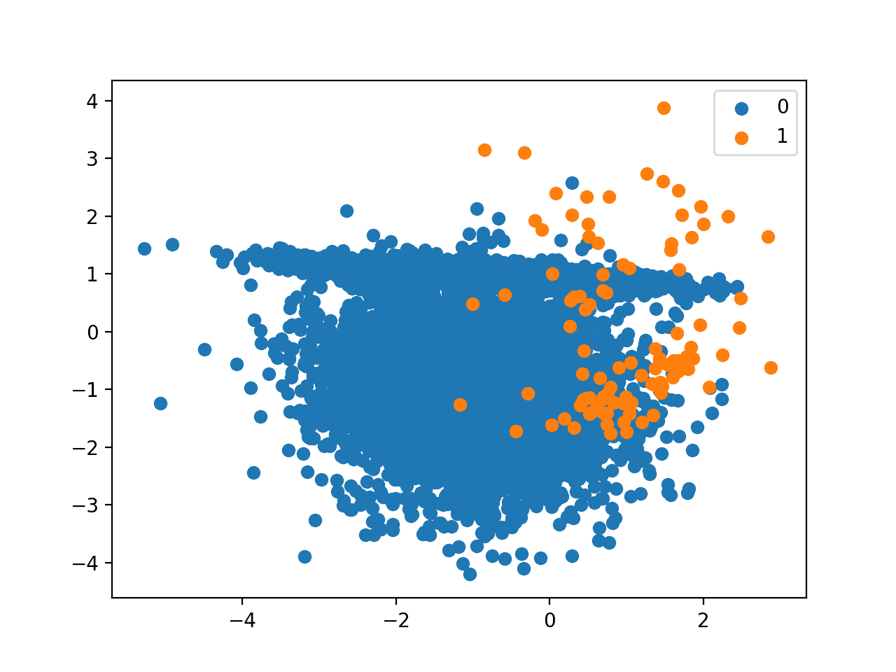
Scatter Plot of Binary Classification Dataset with 1 to 100 Class Imbalance
Want to Get Started With Imbalance Classification?
Take my free 7-day email crash course now (with sample code).
Click to sign-up and also get a free PDF Ebook version of the course.
Neural Network Model in Keras
Next, we can fit a standard neural network model on the dataset.
First, we can define a function to create the synthetic dataset and split it into separate train and test datasets with 5,000 examples in each.
# prepare train and test dataset
def prepare_data():
	# generate 2d classification dataset
	X, y = make_classification(n_samples=10000, n_features=2, n_redundant=0,
	n_clusters_per_class=2, weights=[0.99], flip_y=0, random_state=4)
	# split into train and test
	n_train = 5000
	trainX, testX = X[:n_train, :], X[n_train:, :]
	trainy, testy = y[:n_train], y[n_train:]
	return trainX, trainy, testX, testy
A Multilayer Perceptron neural network can be defined using the Keras deep learning library. We will define a neural network that expects two input variables, has one hidden layer with 10 nodes, then an output layer that predicts the class label.
We will use the popular ReLU activation function in the hidden layer and the sigmoid activation function in the output layer to ensure predictions are probabilities in the range [0,1]. The model will be fit using stochastic gradient descent with the default learning rate and optimized according to cross-entropy loss.
The network architecture and hyperparameters are not optimized to the problem; instead, the network provides a basis for comparison when the training algorithm is later modified to handle the skewed class distribution.
The define_model() function below defines and returns the model, taking the number of input variables to the network as an argument.
# define the neural network model
def define_model(n_input):
	# define model
	model = Sequential()
	# define first hidden layer and visible layer
	model.add(Dense(10, input_dim=n_input, activation='relu', kernel_initializer='he_uniform'))
	# define output layer
	model.add(Dense(1, activation='sigmoid'))
	# define loss and optimizer
	model.compile(loss='binary_crossentropy', optimizer='sgd')
	return model
Once the model is defined, it can be fit on the training dataset.
We will fit the model for 100 training epochs with the default batch size.
...
# fit model
model.fit(trainX, trainy, epochs=100, verbose=0)
Once fit, we can use the model to make predictions on the test dataset, then evaluate the predictions using the ROC AUC score.
...
# make predictions on the test dataset
yhat = model.predict(testX)
# evaluate the ROC AUC of the predictions
score = roc_auc_score(testy, yhat)
print('ROC AUC: %.3f' % score)
Tying this together, the complete example of fitting a standard neural network model on the imbalanced classification dataset is listed below.
# standard neural network on an imbalanced classification dataset
from sklearn.datasets import make_classification
from sklearn.metrics import roc_auc_score
from keras.layers import Dense
from keras.models import Sequential

# prepare train and test dataset
def prepare_data():
	# generate 2d classification dataset
	X, y = make_classification(n_samples=10000, n_features=2, n_redundant=0,
	n_clusters_per_class=2, weights=[0.99], flip_y=0, random_state=4)
	# split into train and test
	n_train = 5000
	trainX, testX = X[:n_train, :], X[n_train:, :]
	trainy, testy = y[:n_train], y[n_train:]
	return trainX, trainy, testX, testy

# define the neural network model
def define_model(n_input):
	# define model
	model = Sequential()
	# define first hidden layer and visible layer
	model.add(Dense(10, input_dim=n_input, activation='relu', kernel_initializer='he_uniform'))
	# define output layer
	model.add(Dense(1, activation='sigmoid'))
	# define loss and optimizer
	model.compile(loss='binary_crossentropy', optimizer='sgd')
	return model

# prepare dataset
trainX, trainy, testX, testy = prepare_data()
# define the model
n_input = trainX.shape[1]
model = define_model(n_input)
# fit model
model.fit(trainX, trainy, epochs=100, verbose=0)
# make predictions on the test dataset
yhat = model.predict(testX)
# evaluate the ROC AUC of the predictions
score = roc_auc_score(testy, yhat)
print('ROC AUC: %.3f' % score)
Running the example evaluates the neural network model on the imbalanced dataset and reports the ROC AUC.
Your specific results may vary given the stochastic nature of the learning algorithm. Try running the example a few times.
In this case, the model achieves a ROC AUC of about 0.949. This suggests that the model has some skill as compared to the naive classifier that has a ROC AUC of 0.5.
ROC AUC: 0.949
This provides a baseline for comparison for any modifications performed to the standard neural network training algorithm.
Deep Learning for Imbalanced Classification
Neural network models are commonly trained using the backpropagation of error algorithm.
This involves using the current state of the model to make predictions for training set examples, calculating the error for the predictions, then updating the model weights using the error, and assigning credit for the error to different nodes and layers backward from the output layer back through to the input layer.
Given the balanced focus on misclassification errors, most standard neural network algorithms are not well suited to datasets with a severely skewed class distribution.
Most of the existing deep learning algorithms do not take the data imbalance problem into consideration. As a result, these algorithms can perform well on the balanced data sets while their performance cannot be guaranteed on imbalanced data sets.
— Training Deep Neural Networks on Imbalanced Data Sets, 2016.
This training procedure can be modified so that some examples have more or less error than others.
The misclassification costs can also be taken in account by changing the error function that is being minimized. Instead of minimizing the squared error, the backpropagation learning procedure should minimize the misclassification costs.
— Cost-Sensitive Learning with Neural Networks, 1998.
The simplest way to implement this is to use a fixed weighting of error scores for examples based on their class where the prediction error is increased for examples in a more important class and decreased or left unchanged for those examples in a less important class.
… cost sensitive learning methods solve data imbalance problem based on the consideration of the cost associated with misclassifying samples. In particular, it assigns different cost values for the misclassification of the samples.
— Training Deep Neural Networks on Imbalanced Data Sets, 2016.
A large error weighting can be applied to those examples in the minority class as they are often more important in an imbalanced classification problem than examples from the majority class.
- Large Weight: Assigned to examples from the minority class.
- Small Weight: Assigned to examples from the majority class.
This modification to the neural network training algorithm is referred to as a Weighted Neural Network or Cost-Sensitive Neural Network.
Typically, careful attention is required when defining the costs or “weightings” to use for cost-sensitive learning. However, for imbalanced classification where only misclassification is the focus, the weighting can use the inverse of the class distribution observed in the training dataset.
Weighted Neural Network With Keras
The Keras Python deep learning library provides support class weighting.
The fit() function that is used to train Keras neural network models takes an argument called class_weight. This argument allows you to define a dictionary that maps class integer values to the importance to apply to each class.
This function is used to train each different type of neural network, including Multilayer Perceptrons, Convolutional Neural Networks, and Recurrent Neural Networks, therefore the class weighting capability is available to all of those network types.
For example, a 1 to 1 weighting for each class 0 and 1 can be defined as follows:
...
# fit model
weights = {0:1, 1:1}
history = model.fit(trainX, trainy, class_weight=weights, ...)
The class weighing can be defined multiple ways; for example:
- Domain expertise, determined by talking to subject matter experts.
- Tuning, determined by a hyperparameter search such as a grid search.
- Heuristic, specified using a general best practice.
A best practice for using the class weighting is to use the inverse of the class distribution present in the training dataset.
For example, the class distribution of the test dataset is a 1:100 ratio for the minority class to the majority class. The invert of this ratio could be used with 1 for the majority class and 100 for the minority class, for example:
...
# fit model
weights = {0:1, 1:100}
history = model.fit(trainX, trainy, class_weight=weights, ...)
Fractions that represent the same ratio do not have the same effect. For example, using 0.01 and 0.99 for the majority and minority classes respectively may result in worse performance than using 1 and 100 (it does in this case).
...
# fit model
weights = {0:0.01, 1:0.99}
history = model.fit(trainX, trainy, class_weight=weights, ...)
The reason is that the error for examples drawn from both the majority class and the minority class is reduced. Further, the reduction in error from the majority class is dramatically scaled down to very small numbers that may have limited or only a very minor effect on model weights.
As such integers are recommended to represent the class weightings, such as 1 for no change and 100 for misclassification errors for class 1 having 100-times more impact or penalty than misclassification errors for class 0.
We can evaluate the neural network algorithm with a class weighting using the same evaluation procedure defined in the previous section.
We would expect the class-weighted version of the neural network to perform better than the version of the training algorithm without any class weighting.
The complete example is listed below.
# class weighted neural network on an imbalanced classification dataset
from sklearn.datasets import make_classification
from sklearn.metrics import roc_auc_score
from keras.layers import Dense
from keras.models import Sequential

# prepare train and test dataset
def prepare_data():
	# generate 2d classification dataset
	X, y = make_classification(n_samples=10000, n_features=2, n_redundant=0,
	n_clusters_per_class=2, weights=[0.99], flip_y=0, random_state=4)
	# split into train and test
	n_train = 5000
	trainX, testX = X[:n_train, :], X[n_train:, :]
	trainy, testy = y[:n_train], y[n_train:]
	return trainX, trainy, testX, testy

# define the neural network model
def define_model(n_input):
	# define model
	model = Sequential()
	# define first hidden layer and visible layer
	model.add(Dense(10, input_dim=n_input, activation='relu', kernel_initializer='he_uniform'))
	# define output layer
	model.add(Dense(1, activation='sigmoid'))
	# define loss and optimizer
	model.compile(loss='binary_crossentropy', optimizer='sgd')
	return model

# prepare dataset
trainX, trainy, testX, testy = prepare_data()
# get the model
n_input = trainX.shape[1]
model = define_model(n_input)
# fit model
weights = {0:1, 1:100}
history = model.fit(trainX, trainy, class_weight=weights, epochs=100, verbose=0)
# evaluate model
yhat = model.predict(testX)
score = roc_auc_score(testy, yhat)
print('ROC AUC: %.3f' % score)
Running the example prepares the synthetic imbalanced classification dataset, then evaluates the class-weighted version of the neural network training algorithm.
Your specific results may vary given the stochastic nature of the learning algorithm. Try running the example a few times.
The ROC AUC score is reported, in this case showing a better score than the unweighted version of the training algorithm, or about 0.973 as compared to about 0.949.
ROC AUC: 0.973
Further Reading
This section provides more resources on the topic if you are looking to go deeper.
Papers
- Cost-Sensitive Learning with Neural Networks, 1998.
- Training Deep Neural Networks on Imbalanced Data Sets, 2016.
Books
- Learning from Imbalanced Data Sets, 2018.
- Imbalanced Learning: Foundations, Algorithms, and Applications, 2013.
APIs
Summary
In this tutorial, you discovered weighted neural networks for imbalanced classification.
Specifically, you learned:
- How the standard neural network algorithm does not support imbalanced classification.
- How the neural network training algorithm can be modified to weight misclassification errors in proportion to class importance.
- How to configure class weight for neural networks and evaluate the effect on model performance.
Do you have any questions?
Ask your questions in the comments below and I will do my best to answer.
The post How to Develop a Cost-Sensitive Neural Network for Imbalanced Classification appeared first on Machine Learning Mastery.