
Author: Jason Brownlee
The XGBoost algorithm is effective for a wide range of regression and classification predictive modeling problems.
It is an efficient implementation of the stochastic gradient boosting algorithm and offers a range of hyperparameters that give fine-grained control over the model training procedure. Although the algorithm performs well in general, even on imbalanced classification datasets, it offers a way to tune the training algorithm to pay more attention to misclassification of the minority class for datasets with a skewed class distribution.
This modified version of XGBoost is referred to as Class Weighted XGBoost or Cost-Sensitive XGBoost and can offer better performance on binary classification problems with a severe class imbalance.
In this tutorial, you will discover weighted XGBoost for imbalanced classification.
After completing this tutorial, you will know:
- How gradient boosting works from a high level and how to develop an XGBoost model for classification.
- How the XGBoost training algorithm can be modified to weight error gradients proportional to positive class importance during training.
- How to configure the positive class weight for the XGBoost training algorithm and how to grid search different configurations.
Discover SMOTE, one-class classification, cost-sensitive learning, threshold moving, and much more in my new book, with 30 step-by-step tutorials and full Python source code.
Let’s get started.

How to Configure XGBoost for Imbalanced Classification
Photo by flowcomm, some rights reserved.
Tutorial Overview
This tutorial is divided into four parts; they are:
- Imbalanced Classification Dataset
- XGBoost Model for Classification
- Weighted XGBoost for Class Imbalance
- Tune the Class Weighting Hyperparameter
Imbalanced Classification Dataset
Before we dive into XGBoost for imbalanced classification, let’s first define an imbalanced classification dataset.
We can use the make_classification() scikit-learn function to define a synthetic imbalanced two-class classification dataset. We will generate 10,000 examples with an approximate 1:100 minority to majority class ratio.
...
# define dataset
X, y = make_classification(n_samples=10000, n_features=2, n_redundant=0,
	n_clusters_per_class=2, weights=[0.99], flip_y=0, random_state=7)
Once generated, we can summarize the class distribution to confirm that the dataset was created as we expected.
...
# summarize class distribution
counter = Counter(y)
print(counter)
Finally, we can create a scatter plot of the examples and color them by class label to help understand the challenge of classifying examples from this dataset.
...
# scatter plot of examples by class label
for label, _ in counter.items():
	row_ix = where(y == label)[0]
	pyplot.scatter(X[row_ix, 0], X[row_ix, 1], label=str(label))
pyplot.legend()
pyplot.show()
Tying this together, the complete example of generating the synthetic dataset and plotting the examples is listed below.
# Generate and plot a synthetic imbalanced classification dataset
from collections import Counter
from sklearn.datasets import make_classification
from matplotlib import pyplot
from numpy import where
# define dataset
X, y = make_classification(n_samples=10000, n_features=2, n_redundant=0,
	n_clusters_per_class=2, weights=[0.99], flip_y=0, random_state=7)
# summarize class distribution
counter = Counter(y)
print(counter)
# scatter plot of examples by class label
for label, _ in counter.items():
	row_ix = where(y == label)[0]
	pyplot.scatter(X[row_ix, 0], X[row_ix, 1], label=str(label))
pyplot.legend()
pyplot.show()
Running the example first creates the dataset and summarizes the class distribution.
We can see that the dataset has an approximate 1:100 class distribution with a little less than 10,000 examples in the majority class and 100 in the minority class.
Counter({0: 9900, 1: 100})
Next, a scatter plot of the dataset is created showing the large mass of examples for the majority class (blue) and a small number of examples for the minority class (orange), with some modest class overlap.
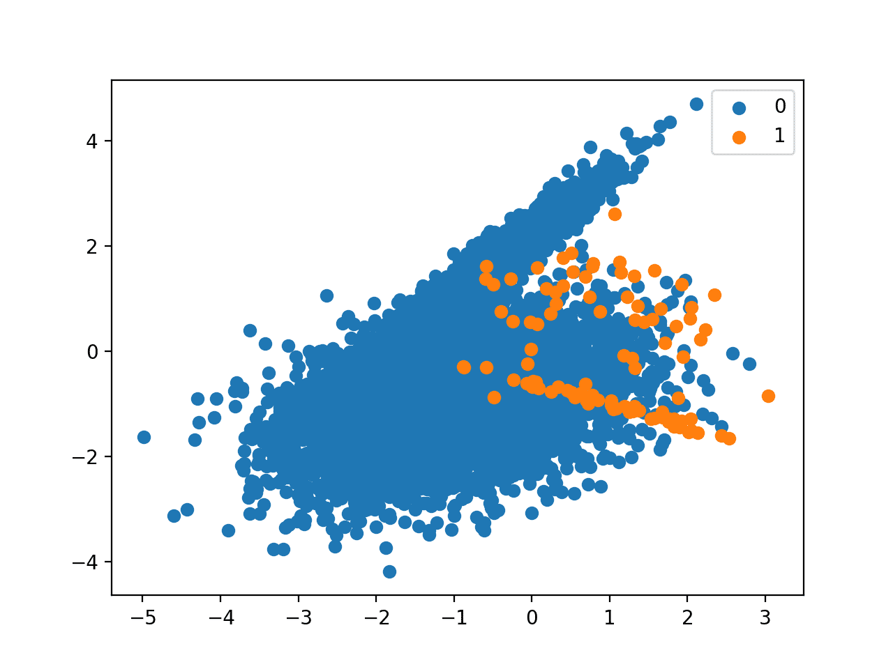
Scatter Plot of Binary Classification Dataset With 1 to 100 Class Imbalance
Want to Get Started With Imbalance Classification?
Take my free 7-day email crash course now (with sample code).
Click to sign-up and also get a free PDF Ebook version of the course.
XGBoost Model for Classification
XGBoost is short for Extreme Gradient Boosting and is an efficient implementation of the stochastic gradient boosting machine learning algorithm.
The stochastic gradient boosting algorithm, also called gradient boosting machines or tree boosting, is a powerful machine learning technique that performs well or even best on a wide range of challenging machine learning problems.
Tree boosting has been shown to give state-of-the-art results on many standard classification benchmarks.
— XGBoost: A Scalable Tree Boosting System, 2016.
It is an ensemble of decision trees algorithm where new trees fix errors of those trees that are already part of the model. Trees are added until no further improvements can be made to the model.
XGBoost provides a highly efficient implementation of the stochastic gradient boosting algorithm and access to a suite of model hyperparameters designed to provide control over the model training process.
The most important factor behind the success of XGBoost is its scalability in all scenarios. The system runs more than ten times faster than existing popular solutions on a single machine and scales to billions of examples in distributed or memory-limited settings.
— XGBoost: A Scalable Tree Boosting System, 2016.
XGBoost is an effective machine learning model, even on datasets where the class distribution is skewed.
Before any modification or tuning is made to the XGBoost algorithm for imbalanced classification, it is important to test the default XGBoost model and establish a baseline in performance.
Although the XGBoost library has its own Python API, we can use XGBoost models with the scikit-learn API via the XGBClassifier wrapper class. An instance of the model can be instantiated and used just like any other scikit-learn class for model evaluation. For example:
...
# define model
model = XGBClassifier()
We will use repeated cross-validation to evaluate the model, with three repeats of 10-fold cross-validation.
The model performance will be reported using the mean ROC area under curve (ROC AUC) averaged over repeats and all folds.
...
# define evaluation procedure
cv = RepeatedStratifiedKFold(n_splits=10, n_repeats=3, random_state=1)
# evaluate model
scores = cross_val_score(model, X, y, scoring='roc_auc', cv=cv, n_jobs=-1)
# summarize performance
print('Mean ROC AUC: %.5f' % mean(scores))
Tying this together, the complete example of defining and evaluating a default XGBoost model on the imbalanced classification problem is listed below.
# fit xgboost on an imbalanced classification dataset
from numpy import mean
from sklearn.datasets import make_classification
from sklearn.model_selection import cross_val_score
from sklearn.model_selection import RepeatedStratifiedKFold
from xgboost import XGBClassifier
# generate dataset
X, y = make_classification(n_samples=10000, n_features=2, n_redundant=0,
	n_clusters_per_class=2, weights=[0.99], flip_y=0, random_state=7)
# define model
model = XGBClassifier()
# define evaluation procedure
cv = RepeatedStratifiedKFold(n_splits=10, n_repeats=3, random_state=1)
# evaluate model
scores = cross_val_score(model, X, y, scoring='roc_auc', cv=cv, n_jobs=-1)
# summarize performance
print('Mean ROC AUC: %.5f' % mean(scores))
Running the example evaluates the default XGBoost model on the imbalanced dataset and reports the mean ROC AUC.
Your specific results may vary given the stochastic nature of the learning algorithm. Try running the example a few times.
We can see that the model has skill, achieving a ROC AUC above 0.5, in this case achieving a mean score of 0.95724.
Mean ROC AUC: 0.95724
This provides a baseline for comparison for any hyperparameter tuning performed for the default XGBoost algorithm.
Weighted XGBoost for Class Imbalance
Although the XGBoost algorithm performs well for a wide range of challenging problems, it offers a large number of hyperparameters, many of which require tuning in order to get the most out of the algorithm on a given dataset.
The implementation provides a hyperparameter designed to tune the behavior of the algorithm for imbalanced classification problems; this is the scale_pos_weight hyperparameter.
By default, the scale_pos_weight hyperparameter is set to the value of 1.0 and has the effect of weighing the balance of positive examples, relative to negative examples when boosting decision trees. For an imbalanced binary classification dataset, the negative class refers to the majority class (class 0) and the positive class refers to the minority class (class 1).
XGBoost is trained to minimize a loss function and the “gradient” in gradient boosting refers to the steepness of this loss function, e.g. the amount of error. A small gradient means a small error and, in turn, a small change to the model to correct the error. A large error gradient during training in turn results in a large correction.
- Small Gradient: Small error or correction to the model.
- Large Gradient: Large error or correction to the model.
Gradients are used as the basis for fitting subsequent trees added to boost or correct errors made by the existing state of the ensemble of decision trees.
The scale_pos_weight value is used to scale the gradient for the positive class.
This has the effect of scaling errors made by the model during training on the positive class and encourages the model to over-correct them. In turn, this can help the model achieve better performance when making predictions on the positive class. Pushed too far, it may result in the model overfitting the positive class at the cost of worse performance on the negative class or both classes.
As such, the scale_pos_weight can be used to train a class-weighted or cost-sensitive version of XGBoost for imbalanced classification.
A sensible default value to set for the scale_pos_weight hyperparameter is the inverse of the class distribution. For example, for a dataset with a 1 to 100 ratio for examples in the minority to majority classes, the scale_pos_weight can be set to 100. This will give classification errors made by the model on the minority class (positive class) 100 times more impact, and in turn, 100 times more correction than errors made on the majority class.
For example:
...
# define model
model = XGBClassifier(scale_pos_weight=100)
The XGBoost documentation suggests a fast way to estimate this value using the training dataset as the total number of examples in the majority class divided by the total number of examples in the minority class.
- scale_pos_weight = total_negative_examples / total_positive_examples
For example, we can calculate this value for our synthetic classification dataset. We would expect this to be about 100, or more precisely, 99 given the weighting we used to define the dataset.
...
# count examples in each class
counter = Counter(y)
# estimate scale_pos_weight value
estimate = counter[0] / counter[1]
print('Estimate: %.3f' % estimate)
The complete example of estimating the value for the scale_pos_weight XGBoost hyperparameter is listed below.
# estimate a value for the scale_pos_weight xgboost hyperparameter
from sklearn.datasets import make_classification
from collections import Counter
# generate dataset
X, y = make_classification(n_samples=10000, n_features=2, n_redundant=0,
	n_clusters_per_class=2, weights=[0.99], flip_y=0, random_state=7)
# count examples in each class
counter = Counter(y)
# estimate scale_pos_weight value
estimate = counter[0] / counter[1]
print('Estimate: %.3f' % estimate)
Running the example creates the dataset and estimates the values of the scale_pos_weight hyperparameter as 99, as we expected.
Estimate: 99.000
We will use this value directly in the configuration of the XGBoost model and evaluate its performance on the dataset using repeated k-fold cross-validation.
We would expect some improvement in ROC AUC, although this is not guaranteed depending on the difficulty of the dataset and the chosen configuration of the XGBoost model.
The complete example is listed below.
# fit balanced xgboost on an imbalanced classification dataset
from numpy import mean
from sklearn.datasets import make_classification
from sklearn.model_selection import cross_val_score
from sklearn.model_selection import RepeatedStratifiedKFold
from xgboost import XGBClassifier
# generate dataset
X, y = make_classification(n_samples=10000, n_features=2, n_redundant=0,
	n_clusters_per_class=2, weights=[0.99], flip_y=0, random_state=7)
# define model
model = XGBClassifier(scale_pos_weight=99)
# define evaluation procedure
cv = RepeatedStratifiedKFold(n_splits=10, n_repeats=3, random_state=1)
# evaluate model
scores = cross_val_score(model, X, y, scoring='roc_auc', cv=cv, n_jobs=-1)
# summarize performance
print('Mean ROC AUC: %.5f' % mean(scores))
Running the example prepares the synthetic imbalanced classification dataset, then evaluates the class-weighted version of the XGBoost training algorithm using repeated cross-validation.
Your specific results may vary given the stochastic nature of the learning algorithm. Try running the example a few times.
In this case, we can see a modest lift in performance from a ROC AUC of about 0.95724 with scale_pos_weight=1 in the previous section to a value of 0.95990 with scale_pos_weight=99.
Mean ROC AUC: 0.95990
Tune the Class Weighting Hyperparameter
The heuristic for setting the scale_pos_weight is effective for many situations.
Nevertheless, it is possible that better performance can be achieved with a different class weighting, and this too will depend on the choice of performance metric used to evaluate the model.
In this section, we will grid search a range of different class weightings for class-weighted XGBoost and discover which results in the best ROC AUC score.
We will try the following weightings for the positive class:
- 1 (default)
- 10
- 25
- 50
- 75
- 99 (recommended)
- 100
- 1000
These can be defined as grid search parameters for the GridSearchCV class as follows:
...
# define grid
weights = [1, 10, 25, 50, 75, 99, 100, 1000]
param_grid = dict(scale_pos_weight=weights)
We can perform the grid search on these parameters using repeated cross-validation and estimate model performance using ROC AUC:
...
# define evaluation procedure
cv = RepeatedStratifiedKFold(n_splits=10, n_repeats=3, random_state=1)
# define grid search
grid = GridSearchCV(estimator=model, param_grid=param_grid, n_jobs=-1, cv=cv, scoring='roc_auc')
Once executed, we can summarize the best configuration as well as all of the results as follows:
...
# report the best configuration
print("Best: %f using %s" % (grid_result.best_score_, grid_result.best_params_))
# report all configurations
means = grid_result.cv_results_['mean_test_score']
stds = grid_result.cv_results_['std_test_score']
params = grid_result.cv_results_['params']
for mean, stdev, param in zip(means, stds, params):
    print("%f (%f) with: %r" % (mean, stdev, param))
Tying this together, the example below grid searches eight different positive class weights for the XGBoost algorithm on the imbalanced dataset.
We might expect that the heuristic class weighing is the best performing configuration.
# grid search positive class weights with xgboost for imbalance classification
from numpy import mean
from sklearn.datasets import make_classification
from sklearn.model_selection import GridSearchCV
from sklearn.model_selection import RepeatedStratifiedKFold
from xgboost import XGBClassifier
# generate dataset
X, y = make_classification(n_samples=10000, n_features=2, n_redundant=0,
	n_clusters_per_class=2, weights=[0.99], flip_y=0, random_state=7)
# define model
model = XGBClassifier()
# define grid
weights = [1, 10, 25, 50, 75, 99, 100, 1000]
param_grid = dict(scale_pos_weight=weights)
# define evaluation procedure
cv = RepeatedStratifiedKFold(n_splits=10, n_repeats=3, random_state=1)
# define grid search
grid = GridSearchCV(estimator=model, param_grid=param_grid, n_jobs=-1, cv=cv, scoring='roc_auc')
# execute the grid search
grid_result = grid.fit(X, y)
# report the best configuration
print("Best: %f using %s" % (grid_result.best_score_, grid_result.best_params_))
# report all configurations
means = grid_result.cv_results_['mean_test_score']
stds = grid_result.cv_results_['std_test_score']
params = grid_result.cv_results_['params']
for mean, stdev, param in zip(means, stds, params):
    print("%f (%f) with: %r" % (mean, stdev, param))
Running the example evaluates each positive class weighting using repeated k-fold cross-validation and reports the best configuration and the associated mean ROC AUC score.
Your specific results may vary given the stochastic nature of the learning algorithm. Try running the example a few times.
In this case, we can see that the scale_pos_weight=99 positive class weighting achieved the best mean ROC score. This matches the configuration for the general heuristic.
It’s interesting to note that almost all values larger than the default value of 1 have a better mean ROC AUC, even the aggressive value of 1,000. It’s also interesting to note that a value of 99 performed better from the value of 100, which I may have used if I did not calculate the heuristic as suggested in the XGBoost documentation.
Best: 0.959901 using {'scale_pos_weight': 99}
0.957239 (0.031619) with: {'scale_pos_weight': 1}
0.958219 (0.027315) with: {'scale_pos_weight': 10}
0.958278 (0.027438) with: {'scale_pos_weight': 25}
0.959199 (0.026171) with: {'scale_pos_weight': 50}
0.959204 (0.025842) with: {'scale_pos_weight': 75}
0.959901 (0.025499) with: {'scale_pos_weight': 99}
0.959141 (0.025409) with: {'scale_pos_weight': 100}
0.958761 (0.024757) with: {'scale_pos_weight': 1000}
Further Reading
This section provides more resources on the topic if you are looking to go deeper.
Papers
Books
- Learning from Imbalanced Data Sets, 2018.
- Imbalanced Learning: Foundations, Algorithms, and Applications, 2013.
APIs
- sklearn.datasets.make_classification API.
- xgboost.XGBClassifier API.
- XGBoost Parameters, API Documentation.
- Notes on Parameter Tuning, API Documentation.
Summary
In this tutorial, you discovered weighted XGBoost for imbalanced classification.
Specifically, you learned:
- How gradient boosting works from a high level and how to develop an XGBoost model for classification.
- How the XGBoost training algorithm can be modified to weight error gradients proportional to positive class importance during training.
- How to configure the positive class weight for the XGBoost training algorithm and how to grid search different configurations.
Do you have any questions?
Ask your questions in the comments below and I will do my best to answer.
The post How to Configure XGBoost for Imbalanced Classification appeared first on Machine Learning Mastery.