Author: Jason Brownlee
Classification predictive modeling typically involves predicting a class label.
Nevertheless, many machine learning algorithms are capable of predicting a probability or scoring of class membership, and this must be interpreted before it can be mapped to a crisp class label. This is achieved by using a threshold, such as 0.5, where all values equal or greater than the threshold are mapped to one class and all other values are mapped to another class.
For those classification problems that have a severe class imbalance, the default threshold can result in poor performance. As such, a simple and straightforward approach to improving the performance of a classifier that predicts probabilities on an imbalanced classification problem is to tune the threshold used to map probabilities to class labels.
In some cases, such as when using ROC Curves and Precision-Recall Curves, the best or optimal threshold for the classifier can be calculated directly. In other cases, it is possible to use a grid search to tune the threshold and locate the optimal value.
In this tutorial, you will discover how to tune the optimal threshold when converting probabilities to crisp class labels for imbalanced classification.
After completing this tutorial, you will know:
- The default threshold for interpreting probabilities to class labels is 0.5, and tuning this hyperparameter is called threshold moving.
- How to calculate the optimal threshold for the ROC Curve and Precision-Recall Curve directly.
- How to manually search threshold values for a chosen model and model evaluation metric.
Discover SMOTE, one-class classification, cost-sensitive learning, threshold moving, and much more in my new book, with 30 step-by-step tutorials and full Python source code.
Let’s get started.
A Gentle Introduction to Threshold-Moving for Imbalanced Classification
Photo by Bruna cs, some rights reserved.
Tutorial Overview
This tutorial is divided into five parts; they are:
- Converting Probabilities to Class Labels
- Threshold-Moving for Imbalanced Classification
- Optimal Threshold for ROC Curve
- Optimal Threshold for Precision-Recall Curve
- Optimal Threshold Tuning
Converting Probabilities to Class Labels
Many machine learning algorithms are capable of predicting a probability or a scoring of class membership.
This is useful generally as it provides a measure of the certainty or uncertainty of a prediction. It also provides additional granularity over just predicting the class label that can be interpreted.
Some classification tasks require a crisp class label prediction. This means that even though a probability or scoring of class membership is predicted, it must be converted into a crisp class label.
The decision for converting a predicted probability or scoring into a class label is governed by a parameter referred to as the “decision threshold,” “discrimination threshold,” or simply the “threshold.” The default value for the threshold is 0.5 for normalized predicted probabilities or scores in the range between 0 or 1.
For example, on a binary classification problem with class labels 0 and 1, normalized predicted probabilities and a threshold of 0.5, then values less than the threshold of 0.5 are assigned to class 0 and values greater than or equal to 0.5 are assigned to class 1.
- Prediction < 0.5 = Class 0
- Prediction >= 0.5 = Class 1
The problem is that the default threshold may not represent an optimal interpretation of the predicted probabilities.
This might be the case for a number of reasons, such as:
- The predicted probabilities are not calibrated, e.g. those predicted by an SVM or decision tree.
- The metric used to train the model is different from the metric used to evaluate a final model.
- The class distribution is severely skewed.
- The cost of one type of misclassification is more important than another type of misclassification.
Worse still, some or all of these reasons may occur at the same time, such as the use of a neural network model with uncalibrated predicted probabilities on an imbalanced classification problem.
As such, there is often the need to change the default decision threshold when interpreting the predictions of a model.
… almost all classifiers generate positive or negative predictions by applying a threshold to a score. The choice of this threshold will have an impact in the trade-offs of positive and negative errors.
— Page 53, Learning from Imbalanced Data Sets, 2018.
Want to Get Started With Imbalance Classification?
Take my free 7-day email crash course now (with sample code).
Click to sign-up and also get a free PDF Ebook version of the course.
Threshold-Moving for Imbalanced Classification
There are many techniques that may be used to address an imbalanced classification problem, such as resampling the training dataset and developing customized version of machine learning algorithms.
Nevertheless, perhaps the simplest approach to handle a severe class imbalance is to change the decision threshold. Although simple and very effective, this technique is often overlooked by practitioners and research academics alike as was noted by Foster Provost in his 2000 article titled “Machine Learning from Imbalanced Data Sets.”
The bottom line is that when studying problems with imbalanced data, using the classifiers produced by standard machine learning algorithms without adjusting the output threshold may well be a critical mistake.
— Machine Learning from Imbalanced Data Sets 101, 2000.
There are many reasons to choose an alternative to the default decision threshold.
For example, you may use ROC curves to analyze the predicted probabilities of a model and ROC AUC scores to compare and select a model, although you require crisp class labels from your model. How do you choose the threshold on the ROC Curve that results in the best balance between the true positive rate and the false positive rate?
Alternately, you may use precision-recall curves to analyze the predicted probabilities of a model, precision-recall AUC to compare and select models, and require crisp class labels as predictions. How do you choose the threshold on the Precision-Recall Curve that results in the best balance between precision and recall?
You may use a probability-based metric to train, evaluate, and compare models like log loss (cross-entropy) but require crisp class labels to be predicted. How do you choose the optimal threshold from predicted probabilities more generally?
Finally, you may have different costs associated with false positive and false negative misclassification, a so-called cost matrix, but wish to use and evaluate cost-insensitive models and later evaluate their predictions use a cost-sensitive measure. How do you choose a threshold that finds the best trade-off for predictions using the cost matrix?
Popular way of training a cost-sensitive classifier without a known cost matrix is to put emphasis on modifying the classification outputs when predictions are being made on new data. This is usually done by setting a threshold on the positive class, below which the negative one is being predicted. The value of this threshold is optimized using a validation set and thus the cost matrix can be learned from training data.
— Page 67, Learning from Imbalanced Data Sets, 2018.
The answer to these questions is to search a range of threshold values in order to find the best threshold. In some cases, the optimal threshold can be calculated directly.
Tuning or shifting the decision threshold in order to accommodate the broader requirements of the classification problem is generally referred to as “threshold-moving,” “threshold-tuning,” or simply “thresholding.”
It has been stated that trying other methods, such as sampling, without trying by simply setting the threshold may be misleading. The threshold-moving method uses the original training set to train [a model] and then moves the decision threshold such that the minority class examples are easier to be predicted correctly.
— Pages 72, Imbalanced Learning: Foundations, Algorithms, and Applications, 2013.
The process involves first fitting the model on a training dataset and making predictions on a test dataset. The predictions are in the form of normalized probabilities or scores that are transformed into normalized probabilities. Different threshold values are then tried and the resulting crisp labels are evaluated using a chosen evaluation metric. The threshold that achieves the best evaluation metric is then adopted for the model when making predictions on new data in the future.
We can summarize this procedure below.
- 1. Fit Model on the Training Dataset.
- 2. Predict Probabilities on the Test Dataset.
- 3. For each threshold in Thresholds:
- 3a. Convert probabilities to Class Labels using the threshold.
- 3b. Evaluate Class Labels.
- 3c. If Score is Better than Best Score.
- 3ci. Adopt Threshold.
- 4. Use Adopted Threshold When Making Class Predictions on New Data.
Although simple, there are a few different approaches to implementing threshold-moving depending on your circumstance. We will take a look at some of the most common examples in the following sections.
Optimal Threshold for ROC Curve
A ROC curve is a diagnostic plot that evaluates a set of probability predictions made by a model on a test dataset.
A set of different thresholds are used to interpret the true positive rate and the false positive rate of the predictions on the positive (minority) class, and the scores are plotted in a line of increasing thresholds to create a curve.
The false-positive rate is plotted on the x-axis and the true positive rate is plotted on the y-axis and the plot is referred to as the Receiver Operating Characteristic curve, or ROC curve. A diagonal line on the plot from the bottom-left to top-right indicates the “curve” for a no-skill classifier (predicts the majority class in all cases), and a point in the top left of the plot indicates a model with perfect skill.
The curve is useful to understand the trade-off in the true-positive rate and false-positive rate for different thresholds. The area under the ROC Curve, so-called ROC AUC, provides a single number to summarize the performance of a model in terms of its ROC Curve with a value between 0.5 (no-skill) and 1.0 (perfect skill).
The ROC Curve is a useful diagnostic tool for understanding the trade-off for different thresholds and the ROC AUC provides a useful number for comparing models based on their general capabilities.
If crisp class labels are required from a model under such an analysis, then an optimal threshold is required. This would be a threshold on the curve that is closest to the top-left of the plot.
Thankfully, there are principled ways of locating this point.
First, let’s fit a model and calculate a ROC Curve.
We can use the make_classification() function to create a synthetic binary classification problem with 10,000 examples (rows), 99 percent of which belong to the majority class and 1 percent belong to the minority class.
...
# generate dataset
X, y = make_classification(n_samples=10000, n_features=2, n_redundant=0,
	n_clusters_per_class=1, weights=[0.99], flip_y=0, random_state=4)
We can then split the dataset using the train_test_split() function and use half for the training set and half for the test set.
...
# split into train/test sets
trainX, testX, trainy, testy = train_test_split(X, y, test_size=0.5, random_state=2, stratify=y)
We can then fit a LogisticRegression model and use it to make probability predictions on the test set and keep only the probability predictions for the minority class.
...
# fit a model
model = LogisticRegression(solver='lbfgs')
model.fit(trainX, trainy)
# predict probabilities
lr_probs = model.predict_proba(testX)
# keep probabilities for the positive outcome only
lr_probs = lr_probs[:, 1]
We can then use the roc_auc_score() function to calculate the true-positive rate and false-positive rate for the predictions using a set of thresholds that can then be used to create a ROC Curve plot.
...
# calculate scores
lr_auc = roc_auc_score(testy, lr_probs)
We can tie this all together, defining the dataset, fitting the model, and creating the ROC Curve plot. The complete example is listed below.
# roc curve for logistic regression model
from sklearn.datasets import make_classification
from sklearn.linear_model import LogisticRegression
from sklearn.model_selection import train_test_split
from sklearn.metrics import roc_curve
from matplotlib import pyplot
# generate dataset
X, y = make_classification(n_samples=10000, n_features=2, n_redundant=0,
	n_clusters_per_class=1, weights=[0.99], flip_y=0, random_state=4)
# split into train/test sets
trainX, testX, trainy, testy = train_test_split(X, y, test_size=0.5, random_state=2, stratify=y)
# fit a model
model = LogisticRegression(solver='lbfgs')
model.fit(trainX, trainy)
# predict probabilities
yhat = model.predict_proba(testX)
# keep probabilities for the positive outcome only
yhat = yhat[:, 1]
# calculate roc curves
fpr, tpr, thresholds = roc_curve(testy, yhat)
# plot the roc curve for the model
pyplot.plot([0,1], [0,1], linestyle='--', label='No Skill')
pyplot.plot(fpr, tpr, marker='.', label='Logistic')
# axis labels
pyplot.xlabel('False Positive Rate')
pyplot.ylabel('True Positive Rate')
pyplot.legend()
# show the plot
pyplot.show()
Running the example fits a logistic regression model on the training dataset then evaluates it using a range of thresholds on the test set, creating the ROC Curve
We can see that there are a number of points or thresholds close to the top-left of the plot.
Which is the threshold that is optimal?
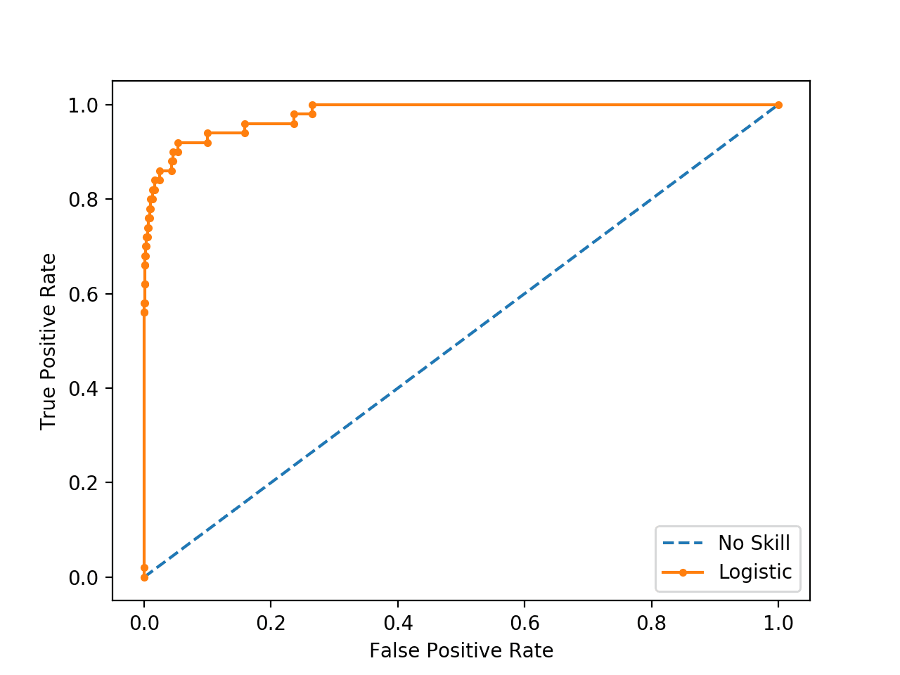
ROC Curve Line Plot for Logistic Regression Model for Imbalanced Classification
There are many ways we could locate the threshold with the optimal balance between false positive and true positive rates.
Firstly, the true positive rate is called the Sensitivity. The inverse of the false-positive rate is called the Specificity.
- Sensitivity = TruePositive / (TruePositive + FalseNegative)
- Specificity = FalseNegative / (FalsePositive + TrueNegative)
Where:
- Sensitivity = True Positive Rate
- Specificity = 1 – False Positive Rate
The Geometric Mean or G-Mean is a metric for imbalanced classification that, if optimized, will seek a balance between the sensitivity and the specificity.
- G-Mean = sqrt(Sensitivity * Specificity)
One approach would be to test the model with each threshold returned from the call roc_auc_score() and select the threshold with the largest G-Mean value.
Given that we have already calculated the Sensitivity (TPR) and the complement to the Specificity when we calculated the ROC Curve, we can calculate the G-Mean for each threshold directly.
...
# calculate the g-mean for each threshold
gmeans = sqrt(tpr * (1-fpr))
Once calculated, we can locate the index for the largest G-mean score and use that index to determine which threshold value to use.
...
# locate the index of the largest g-mean
ix = argmax(gmeans)
print('Best Threshold=%f, G-Mean=%.3f' % (thresholds[ix], gmeans[ix]))
We can also re-draw the ROC Curve and highlight this point.
The complete example is listed below.
# roc curve for logistic regression model with optimal threshold
from numpy import sqrt
from numpy import argmax
from sklearn.datasets import make_classification
from sklearn.linear_model import LogisticRegression
from sklearn.model_selection import train_test_split
from sklearn.metrics import roc_curve
from matplotlib import pyplot
# generate dataset
X, y = make_classification(n_samples=10000, n_features=2, n_redundant=0,
	n_clusters_per_class=1, weights=[0.99], flip_y=0, random_state=4)
# split into train/test sets
trainX, testX, trainy, testy = train_test_split(X, y, test_size=0.5, random_state=2, stratify=y)
# fit a model
model = LogisticRegression(solver='lbfgs')
model.fit(trainX, trainy)
# predict probabilities
yhat = model.predict_proba(testX)
# keep probabilities for the positive outcome only
yhat = yhat[:, 1]
# calculate roc curves
fpr, tpr, thresholds = roc_curve(testy, yhat)
# calculate the g-mean for each threshold
gmeans = sqrt(tpr * (1-fpr))
# locate the index of the largest g-mean
ix = argmax(gmeans)
print('Best Threshold=%f, G-Mean=%.3f' % (thresholds[ix], gmeans[ix]))
# plot the roc curve for the model
pyplot.plot([0,1], [0,1], linestyle='--', label='No Skill')
pyplot.plot(fpr, tpr, marker='.', label='Logistic')
pyplot.scatter(fpr[ix], tpr[ix], marker='o', color='black', label='Best')
# axis labels
pyplot.xlabel('False Positive Rate')
pyplot.ylabel('True Positive Rate')
pyplot.legend()
# show the plot
pyplot.show()
Running the example first locates the optimal threshold and reports this threshold and the G-Mean score.
In this case, we can see that the optimal threshold is about 0.016153.
Best Threshold=0.016153, G-Mean=0.933
The threshold is then used to locate the true and false positive rates, then this point is drawn on the ROC Curve.
We can see that the point for the optimal threshold is a large black dot and it appears to be closest to the top-left of the plot.
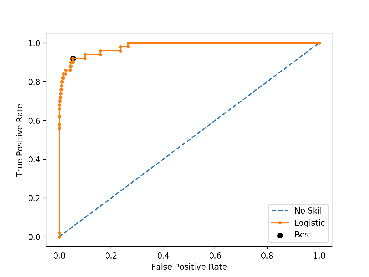
ROC Curve Line Plot for Logistic Regression Model for Imbalanced Classification With the Optimal Threshold
It turns out there is a much faster way to get the same result, called the Youden’s J statistic.
The statistic is calculated as:
- J = Sensitivity + Specificity – 1
Given that we have Sensitivity (TPR) and the complement of the specificity (FPR), we can calculate it as:
- J = Sensitivity + (1 – FalsePositiveRate) – 1
Which we can restate as:
- J = TruePositiveRate – FalsePositiveRate
We can then choose the threshold with the largest J statistic value. For example:
...
# calculate roc curves
fpr, tpr, thresholds = roc_curve(testy, yhat)
# get the best threshold
J = tpr - fpr
ix = argmax(J)
best_thresh = thresholds[ix]
print('Best Threshold=%f' % (best_thresh))
Plugging this in, the complete example is listed below.
# roc curve for logistic regression model with optimal threshold
from numpy import argmax
from sklearn.datasets import make_classification
from sklearn.linear_model import LogisticRegression
from sklearn.model_selection import train_test_split
from sklearn.metrics import roc_curve
# generate dataset
X, y = make_classification(n_samples=10000, n_features=2, n_redundant=0,
	n_clusters_per_class=1, weights=[0.99], flip_y=0, random_state=4)
# split into train/test sets
trainX, testX, trainy, testy = train_test_split(X, y, test_size=0.5, random_state=2, stratify=y)
# fit a model
model = LogisticRegression(solver='lbfgs')
model.fit(trainX, trainy)
# predict probabilities
yhat = model.predict_proba(testX)
# keep probabilities for the positive outcome only
yhat = yhat[:, 1]
# calculate roc curves
fpr, tpr, thresholds = roc_curve(testy, yhat)
# get the best threshold
J = tpr - fpr
ix = argmax(J)
best_thresh = thresholds[ix]
print('Best Threshold=%f' % (best_thresh))
We can see that this simpler approach calculates the optimal statistic directly.
Best Threshold=0.016153
Optimal Threshold for Precision-Recall Curve
Unlike the ROC Curve, a precision-recall curve focuses on the performance of a classifier on the positive (minority class) only.
Precision is the ratio of the number of true positives divided by the sum of the true positives and false positives. It describes how good a model is at predicting the positive class. Recall is calculated as the ratio of the number of true positives divided by the sum of the true positives and the false negatives. Recall is the same as sensitivity.
A precision-recall curve is calculated by creating crisp class labels for probability predictions across a set of thresholds and calculating the precision and recall for each threshold. A line plot is created for the thresholds in ascending order with recall on the x-axis and precision on the y-axis.
A no-skill model is represented by a horizontal line with a precision that is the ratio of positive examples in the dataset (e.g. TP / (TP + TN)), or 0.01 on our synthetic dataset. perfect skill classifier has full precision and recall with a dot in the top-right corner.
We can use the same model and dataset from the previous section and evaluate the probability predictions for a logistic regression model using a precision-recall curve. The precision_recall_curve() function can be used to calculate the curve, returning the precision and recall scores for each threshold as well as the thresholds used.
...
# calculate pr-curve
precision, recall, thresholds = precision_recall_curve(testy, yhat)
Tying this together, the complete example of calculating a precision-recall curve for a logistic regression on an imbalanced classification problem is listed below.
# pr curve for logistic regression model
from sklearn.datasets import make_classification
from sklearn.linear_model import LogisticRegression
from sklearn.model_selection import train_test_split
from sklearn.metrics import precision_recall_curve
from matplotlib import pyplot
# generate dataset
X, y = make_classification(n_samples=10000, n_features=2, n_redundant=0,
	n_clusters_per_class=1, weights=[0.99], flip_y=0, random_state=4)
# split into train/test sets
trainX, testX, trainy, testy = train_test_split(X, y, test_size=0.5, random_state=2, stratify=y)
# fit a model
model = LogisticRegression(solver='lbfgs')
model.fit(trainX, trainy)
# predict probabilities
yhat = model.predict_proba(testX)
# keep probabilities for the positive outcome only
yhat = yhat[:, 1]
# calculate pr-curve
precision, recall, thresholds = precision_recall_curve(testy, yhat)
# plot the roc curve for the model
no_skill = len(testy[testy==1]) / len(testy)
pyplot.plot([0,1], [no_skill,no_skill], linestyle='--', label='No Skill')
pyplot.plot(recall, precision, marker='.', label='Logistic')
# axis labels
pyplot.xlabel('Recall')
pyplot.ylabel('Precision')
pyplot.legend()
# show the plot
pyplot.show()
Running the example calculates the precision and recall for each threshold and creates a precision-recall plot showing that the model has some skill across a range of thresholds on this dataset.
If we required crisp class labels from this model, which threshold would achieve the best result?
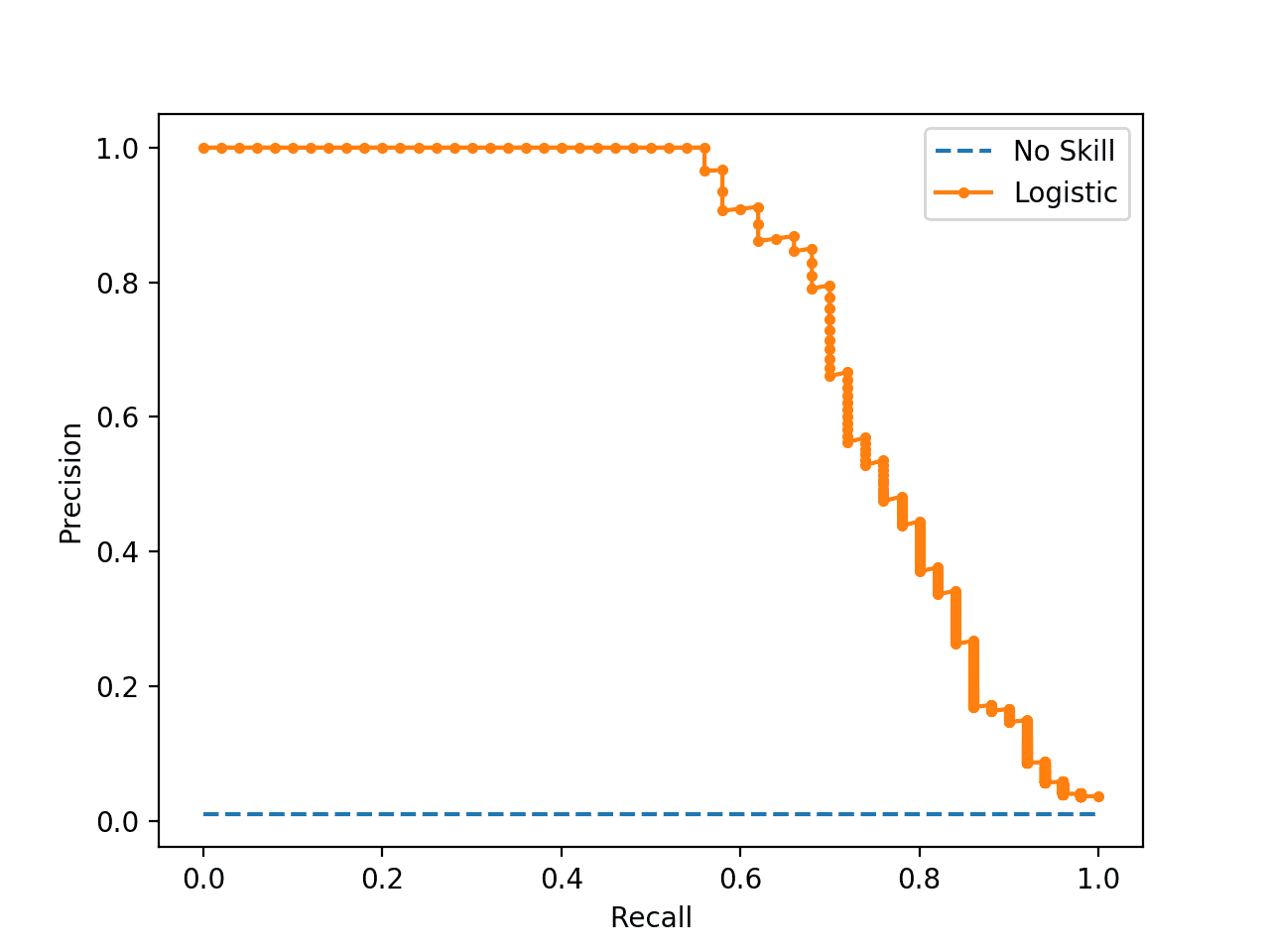
Precision-Recall Curve Line Plot for Logistic Regression Model for Imbalanced Classification
If we are interested in a threshold that results in the best balance of precision and recall, then this is the same as optimizing the F-measure that summarizes the harmonic mean of both measures.
- F-Measure = (2 * Precision * Recall) / (Precision + Recall)
As in the previous section, the naive approach to finding the optimal threshold would be to calculate the F-measure for each threshold. We can achieve the same effect by converting the precision and recall measures to F-measure directly; for example:
...
# convert to f score
fscore = (2 * precision * recall) / (precision + recall)
# locate the index of the largest f score
ix = argmax(fscore)
print('Best Threshold=%f, F-Score=%.3f' % (thresholds[ix], fscore[ix]))
We can then plot the point on the precision-recall curve.
The complete example is listed below.
# optimal threshold for precision-recall curve with logistic regression model
from numpy import argmax
from sklearn.datasets import make_classification
from sklearn.linear_model import LogisticRegression
from sklearn.model_selection import train_test_split
from sklearn.metrics import precision_recall_curve
from matplotlib import pyplot
# generate dataset
X, y = make_classification(n_samples=10000, n_features=2, n_redundant=0,
	n_clusters_per_class=1, weights=[0.99], flip_y=0, random_state=4)
# split into train/test sets
trainX, testX, trainy, testy = train_test_split(X, y, test_size=0.5, random_state=2, stratify=y)
# fit a model
model = LogisticRegression(solver='lbfgs')
model.fit(trainX, trainy)
# predict probabilities
yhat = model.predict_proba(testX)
# keep probabilities for the positive outcome only
yhat = yhat[:, 1]
# calculate roc curves
precision, recall, thresholds = precision_recall_curve(testy, yhat)
# convert to f score
fscore = (2 * precision * recall) / (precision + recall)
# locate the index of the largest f score
ix = argmax(fscore)
print('Best Threshold=%f, F-Score=%.3f' % (thresholds[ix], fscore[ix]))
# plot the roc curve for the model
no_skill = len(testy[testy==1]) / len(testy)
pyplot.plot([0,1], [no_skill,no_skill], linestyle='--', label='No Skill')
pyplot.plot(recall, precision, marker='.', label='Logistic')
pyplot.scatter(recall[ix], precision[ix], marker='o', color='black', label='Best')
# axis labels
pyplot.xlabel('Recall')
pyplot.ylabel('Precision')
pyplot.legend()
# show the plot
pyplot.show()
Running the example first calculates the F-measure for each threshold, then locates the score and threshold with the largest value.
In this case, we can see that the best F-measure was 0.756 achieved with a threshold of about 0.25.
Best Threshold=0.256036, F-Score=0.756
The precision-recall curve is plotted, and this time the threshold with the optimal F-measure is plotted with a larger black dot.
This threshold could then be used when making probability predictions in the future that must be converted from probabilities to crisp class labels.
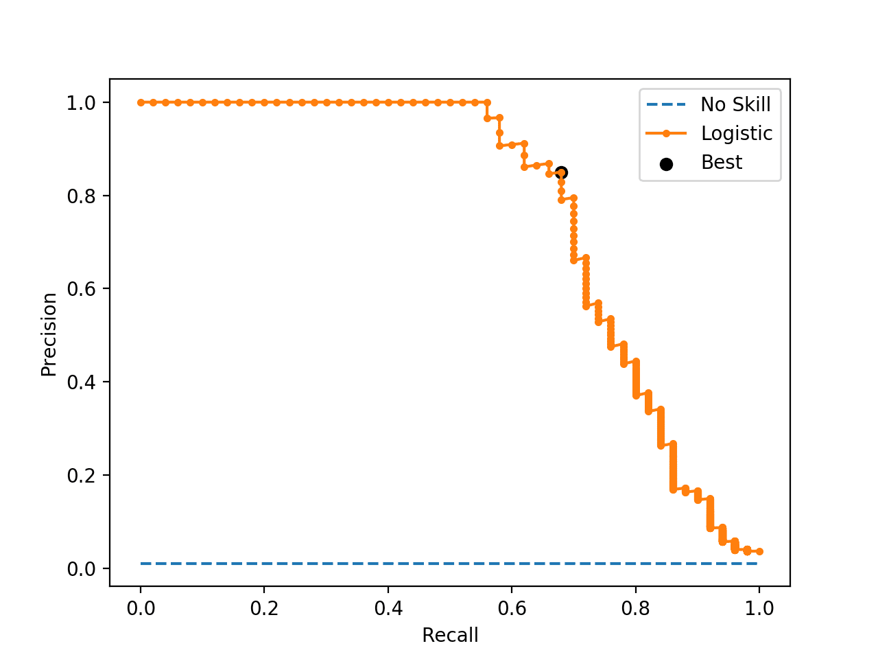
Precision-Recall Curve Line Plot for Logistic Regression Model With Optimal Threshold
Optimal Threshold Tuning
Sometimes, we simply have a model and we wish to know the best threshold directly.
In this case, we can define a set of thresholds and then evaluate predicted probabilities under each in order to find and select the optimal threshold.
We can demonstrate this with a worked example.
First, we can fit a logistic regression model on our synthetic classification problem, then predict class labels and evaluate them using the F-Measure, which is the harmonic mean of precision and recall.
This will use the default threshold of 0.5 when interpreting the probabilities predicted by the logistic regression model.
The complete example is listed below.
# logistic regression for imbalanced classification
from sklearn.datasets import make_classification
from sklearn.linear_model import LogisticRegression
from sklearn.model_selection import train_test_split
from sklearn.metrics import f1_score
# generate dataset
X, y = make_classification(n_samples=10000, n_features=2, n_redundant=0,
	n_clusters_per_class=1, weights=[0.99], flip_y=0, random_state=4)
# split into train/test sets
trainX, testX, trainy, testy = train_test_split(X, y, test_size=0.5, random_state=2, stratify=y)
# fit a model
model = LogisticRegression(solver='lbfgs')
model.fit(trainX, trainy)
# predict labels
yhat = model.predict(testX)
# evaluate the model
score = f1_score(testy, yhat)
print('F-Score: %.5f' % score)
Running the example, we can see that the model achieved an F-Measure of about 0.70 on the test dataset.
F-Score: 0.70130
Now we can use the same model on the same dataset and instead of predicting class labels directly, we can predict probabilities.
...
# predict probabilities
yhat = model.predict_proba(testX)
We only require the probabilities for the positive class.
...
# keep probabilities for the positive outcome only
probs = yhat[:, 1]
Next, we can then define a set of thresholds to evaluate the probabilities. In this case, we will test all thresholds between 0.0 and 1.0 with a step size of 0.001, that is, we will test 0.0, 0.001, 0.002, 0.003, and so on to 0.999.
...
# define thresholds
thresholds = arange(0, 1, 0.001)
Next, we need a way of using a single threshold to interpret the predicted probabilities.
This can be achieved by mapping all values equal to or greater than the threshold to 1 and all values less than the threshold to 0. We will define a to_labels() function to do this that will take the probabilities and threshold as an argument and return an array of integers in {0, 1}.
# apply threshold to positive probabilities to create labels
def to_labels(pos_probs, threshold):
	return (pos_probs >= threshold).astype('int')
We can then call this function for each threshold and evaluate the resulting labels using the f1_score().
We can do this in a single line, as follows:
...
# evaluate each threshold
scores = [f1_score(testy, to_labels(probs, t)) for t in thresholds]
We now have an array of scores that evaluate each threshold in our array of thresholds.
All we need to do now is locate the array index that has the largest score (best F-Measure) and we will have the optimal threshold and its evaluation.
...
# get best threshold
ix = argmax(scores)
print('Threshold=%.3f, F-Score=%.5f' % (thresholds[ix], scores[ix]))
Tying this all together, the complete example of tuning the threshold for the logistic regression model on the synthetic imbalanced classification dataset is listed below.
# search thresholds for imbalanced classification
from numpy import arange
from numpy import argmax
from sklearn.datasets import make_classification
from sklearn.linear_model import LogisticRegression
from sklearn.model_selection import train_test_split
from sklearn.metrics import f1_score

# apply threshold to positive probabilities to create labels
def to_labels(pos_probs, threshold):
	return (pos_probs >= threshold).astype('int')

# generate dataset
X, y = make_classification(n_samples=10000, n_features=2, n_redundant=0,
	n_clusters_per_class=1, weights=[0.99], flip_y=0, random_state=4)
# split into train/test sets
trainX, testX, trainy, testy = train_test_split(X, y, test_size=0.5, random_state=2, stratify=y)
# fit a model
model = LogisticRegression(solver='lbfgs')
model.fit(trainX, trainy)
# predict probabilities
yhat = model.predict_proba(testX)
# keep probabilities for the positive outcome only
probs = yhat[:, 1]
# define thresholds
thresholds = arange(0, 1, 0.001)
# evaluate each threshold
scores = [f1_score(testy, to_labels(probs, t)) for t in thresholds]
# get best threshold
ix = argmax(scores)
print('Threshold=%.3f, F-Score=%.5f' % (thresholds[ix], scores[ix]))
Running the example reports the optimal threshold as 0.251 (compared to the default of 0.5) that achieves an F-Measure of about 0.75 (compared to 0.70).
You can use this example as a template when tuning the threshold on your own problem, allowing you to substitute your own model, metric, and even resolution of thresholds that you want to evaluate.
Threshold=0.251, F-Score=0.75556
Further Reading
This section provides more resources on the topic if you are looking to go deeper.
Papers
- Machine Learning from Imbalanced Data Sets 101, 2000.
- Training Cost-sensitive Neural Networks With Methods Addressing The Class Imbalance Problem, 2005.
Books
- Learning from Imbalanced Data Sets, 2018.
- Imbalanced Learning: Foundations, Algorithms, and Applications, 2013.
APIs
- sklearn.metrics.roc_curve API.
- imblearn.metrics.geometric_mean_score API.
- sklearn.metrics.precision_recall_curve API.
Articles
- Discrimination Threshold, Yellowbrick.
- Youden’s J statistic, Wikipedia.
- Receiver operating characteristic, Wikipedia.
Summary
In this tutorial, you discovered how to tune the optimal threshold when converting probabilities to crisp class labels for imbalanced classification.
Specifically, you learned:
- The default threshold for interpreting probabilities to class labels is 0.5, and tuning this hyperparameter is called threshold moving.
- How to calculate the optimal threshold for the ROC Curve and Precision-Recall Curve directly.
- How to manually search threshold values for a chosen model and model evaluation metric.
Do you have any questions?
Ask your questions in the comments below and I will do my best to answer.
The post A Gentle Introduction to Threshold-Moving for Imbalanced Classification appeared first on Machine Learning Mastery.