
Author: Jason Brownlee
Datasets may have missing values, and this can cause problems for many machine learning algorithms.
As such, it is good practice to identify and replace missing values for each column in your input data prior to modeling your prediction task. This is called missing data imputation, or imputing for short.
A popular approach to missing data imputation is to use a model to predict the missing values. This requires a model to be created for each input variable that has missing values. Although any one among a range of different models can be used to predict the missing values, the k-nearest neighbor (KNN) algorithm has proven to be generally effective, often referred to as “nearest neighbor imputation.”
In this tutorial, you will discover how to use nearest neighbor imputation strategies for missing data in machine learning.
After completing this tutorial, you will know:
- Missing values must be marked with NaN values and can be replaced with nearest neighbor estimated values.
- How to load a CSV file with missing values and mark the missing values with NaN values and report the number and percentage of missing values for each column.
- How to impute missing values with nearest neighbor models as a data preparation method when evaluating models and when fitting a final model to make predictions on new data.
Let’s get started.

kNN Imputation for Missing Values in Machine Learning
Photo by portengaround, some rights reserved.
Tutorial Overview
This tutorial is divided into three parts; they are:
- k-Nearest Neighbor Imputation
- Horse Colic Dataset
- Nearest Neighbor Imputation With KNNImputer
- KNNImputer Data Transform
- KNNImputer and Model Evaluation
- KNNImputer and Different Number of Neighbors
- KNNImputer Transform When Making a Prediction
k-Nearest Neighbor Imputation
A dataset may have missing values.
These are rows of data where one or more values or columns in that row are not present. The values may be missing completely or they may be marked with a special character or value, such as a question mark “?“.
Values could be missing for many reasons, often specific to the problem domain, and might include reasons such as corrupt measurements or unavailability.
Most machine learning algorithms require numeric input values, and a value to be present for each row and column in a dataset. As such, missing values can cause problems for machine learning algorithms.
It is common to identify missing values in a dataset and replace them with a numeric value. This is called data imputing, or missing data imputation.
… missing data can be imputed. In this case, we can use information in the training set predictors to, in essence, estimate the values of other predictors.
— Page 42, Applied Predictive Modeling, 2013.
An effective approach to data imputing is to use a model to predict the missing values. A model is created for each feature that has missing values, taking as input values of perhaps all other input features.
One popular technique for imputation is a K-nearest neighbor model. A new sample is imputed by finding the samples in the training set “closest” to it and averages these nearby points to fill in the value.
— Page 42, Applied Predictive Modeling, 2013.
If input variables are numeric, then regression models can be used for prediction, and this case is quite common. A range of different models can be used, although a simple k-nearest neighbor (KNN) model has proven to be effective in experiments. The use of a KNN model to predict or fill missing values is referred to as “Nearest Neighbor Imputation” or “KNN imputation.”
We show that KNNimpute appears to provide a more robust and sensitive method for missing value estimation […] and KNNimpute surpass the commonly used row average method (as well as filling missing values with zeros).
— Missing value estimation methods for DNA microarrays, 2001.
Configuration of KNN imputation often involves selecting the distance measure (e.g. Euclidean) and the number of contributing neighbors for each prediction, the k hyperparameter of the KNN algorithm.
Now that we are familiar with nearest neighbor methods for missing value imputation, let’s take a look at a dataset with missing values.
Horse Colic Dataset
The horse colic dataset describes medical characteristics of horses with colic and whether they lived or died.
There are 300 rows and 26 input variables with one output variable. It is a binary classification prediction task that involves predicting 1 if the horse lived and 2 if the horse died.
A naive model can achieve a classification accuracy of about 67 percent, and a top-performing model can achieve an accuracy of about 85.2 percent using three repeats of 10-fold cross-validation. This defines the range of expected modeling performance on the dataset.
The dataset has many missing values for many of the columns where each missing value is marked with a question mark character (“?”).
Below provides an example of rows from the dataset with marked missing values.
2,1,530101,38.50,66,28,3,3,?,2,5,4,4,?,?,?,3,5,45.00,8.40,?,?,2,2,11300,00000,00000,2
1,1,534817,39.2,88,20,?,?,4,1,3,4,2,?,?,?,4,2,50,85,2,2,3,2,02208,00000,00000,2
2,1,530334,38.30,40,24,1,1,3,1,3,3,1,?,?,?,1,1,33.00,6.70,?,?,1,2,00000,00000,00000,1
1,9,5290409,39.10,164,84,4,1,6,2,2,4,4,1,2,5.00,3,?,48.00,7.20,3,5.30,2,1,02208,00000,00000,1
...
You can learn more about the dataset here:
No need to download the dataset as we will download it automatically in the worked examples.
Marking missing values with a NaN (not a number) value in a loaded dataset using Python is a best practice.
We can load the dataset using the read_csv() Pandas function and specify the “na_values” to load values of ‘?’ as missing, marked with a NaN value.
...
# load dataset
url = 'https://raw.githubusercontent.com/jbrownlee/Datasets/master/horse-colic.csv'
dataframe = read_csv(url, header=None, na_values='?')
Once loaded, we can review the loaded data to confirm that “?” values are marked as NaN.
...
# summarize the first few rows
print(dataframe.head())
We can then enumerate each column and report the number of rows with missing values for the column.
...
# summarize the number of rows with missing values for each column
for i in range(dataframe.shape[1]):
	# count number of rows with missing values
	n_miss = dataframe[[i]].isnull().sum()
	perc = n_miss / dataframe.shape[0] * 100
	print('> %d, Missing: %d (%.1f%%)' % (i, n_miss, perc))
Tying this together, the complete example of loading and summarizing the dataset is listed below.
# summarize the horse colic dataset
from pandas import read_csv
# load dataset
url = 'https://raw.githubusercontent.com/jbrownlee/Datasets/master/horse-colic.csv'
dataframe = read_csv(url, header=None, na_values='?')
# summarize the first few rows
print(dataframe.head())
# summarize the number of rows with missing values for each column
for i in range(dataframe.shape[1]):
	# count number of rows with missing values
	n_miss = dataframe[[i]].isnull().sum()
	perc = n_miss / dataframe.shape[0] * 100
	print('> %d, Missing: %d (%.1f%%)' % (i, n_miss, perc))
Running the example first loads the dataset and summarizes the first five rows.
We can see that the missing values that were marked with a “?” character have been replaced with NaN values.
0   1        2     3      4     5    6   ...   21   22  23     24  25  26  27
0  2.0   1   530101  38.5   66.0  28.0  3.0  ...  NaN  2.0   2  11300   0   0   2
1  1.0   1   534817  39.2   88.0  20.0  NaN  ...  2.0  3.0   2   2208   0   0   2
2  2.0   1   530334  38.3   40.0  24.0  1.0  ...  NaN  1.0   2      0   0   0   1
3  1.0   9  5290409  39.1  164.0  84.0  4.0  ...  5.3  2.0   1   2208   0   0   1
4  2.0   1   530255  37.3  104.0  35.0  NaN  ...  NaN  2.0   2   4300   0   0   2

[5 rows x 28 columns]
Next, we can see a list of all columns in the dataset and the number and percentage of missing values.
We can see that some columns (e.g. column indexes 1 and 2) have no missing values and other columns (e.g. column indexes 15 and 21) have many or even a majority of missing values.
> 0, Missing: 1 (0.3%)
> 1, Missing: 0 (0.0%)
> 2, Missing: 0 (0.0%)
> 3, Missing: 60 (20.0%)
> 4, Missing: 24 (8.0%)
> 5, Missing: 58 (19.3%)
> 6, Missing: 56 (18.7%)
> 7, Missing: 69 (23.0%)
> 8, Missing: 47 (15.7%)
> 9, Missing: 32 (10.7%)
> 10, Missing: 55 (18.3%)
> 11, Missing: 44 (14.7%)
> 12, Missing: 56 (18.7%)
> 13, Missing: 104 (34.7%)
> 14, Missing: 106 (35.3%)
> 15, Missing: 247 (82.3%)
> 16, Missing: 102 (34.0%)
> 17, Missing: 118 (39.3%)
> 18, Missing: 29 (9.7%)
> 19, Missing: 33 (11.0%)
> 20, Missing: 165 (55.0%)
> 21, Missing: 198 (66.0%)
> 22, Missing: 1 (0.3%)
> 23, Missing: 0 (0.0%)
> 24, Missing: 0 (0.0%)
> 25, Missing: 0 (0.0%)
> 26, Missing: 0 (0.0%)
> 27, Missing: 0 (0.0%)
Now that we are familiar with the horse colic dataset that has missing values, let’s look at how we can use nearest neighbor imputation.
Nearest Neighbor Imputation with KNNImputer
The scikit-learn machine learning library provides the KNNImputer class that supports nearest neighbor imputation.
In this section, we will explore how to effectively use the KNNImputer class.
KNNImputer Data Transform
KNNImputer is a data transform that is first configured based on the method used to estimate the missing values.
The default distance measure is a Euclidean distance measure that is NaN aware, e.g. will not include NaN values when calculating the distance between members of the training dataset. This is set via the “metric” argument.
The number of neighbors is set to five by default and can be configured by the “n_neighbors” argument.
Finally, the distance measure can be weighed proportional to the distance between instances (rows), although this is set to a uniform weighting by default, controlled via the “weights” argument.
...
# define imputer
imputer = KNNImputer(n_neighbors=5, weights='uniform', metric='nan_euclidean')
Then, the imputer is fit on a dataset.
...
# fit on the dataset
imputer.fit(X)
Then, the fit imputer is applied to a dataset to create a copy of the dataset with all missing values for each column replaced with an estimated value.
...
# transform the dataset
Xtrans = imputer.transform(X)
We can demonstrate its usage on the horse colic dataset and confirm it works by summarizing the total number of missing values in the dataset before and after the transform.
The complete example is listed below.
# knn imputation transform for the horse colic dataset
from numpy import isnan
from pandas import read_csv
from sklearn.impute import KNNImputer
# load dataset
url = 'https://raw.githubusercontent.com/jbrownlee/Datasets/master/horse-colic.csv'
dataframe = read_csv(url, header=None, na_values='?')
# split into input and output elements
data = dataframe.values
X, y = data[:, :-1], data[:, -1]
# print total missing
print('Missing: %d' % sum(isnan(X).flatten()))
# define imputer
imputer = KNNImputer()
# fit on the dataset
imputer.fit(X)
# transform the dataset
Xtrans = imputer.transform(X)
# print total missing
print('Missing: %d' % sum(isnan(Xtrans).flatten()))
Running the example first loads the dataset and reports the total number of missing values in the dataset as 1,605.
The transform is configured, fit, and performed, and the resulting new dataset has no missing values, confirming it was performed as we expected.
Each missing value was replaced with a value estimated by the model.
Missing: 1605
Missing: 0
KNNImputer and Model Evaluation
It is a good practice to evaluate machine learning models on a dataset using k-fold cross-validation.
To correctly apply nearest neighbor missing data imputation and avoid data leakage, it is required that the models are calculated for each column are calculated on the training dataset only, then applied to the train and test sets for each fold in the dataset.
This can be achieved by creating a modeling pipeline where the first step is the nearest neighbor imputation, then the second step is the model. This can be achieved using the Pipeline class.
For example, the Pipeline below uses a KNNImputer with the default strategy, followed by a random forest model.
...
# define modeling pipeline
model = RandomForestClassifier()
imputer = KNNImputer()
pipeline = Pipeline(steps=[('i', imputer), ('m', model)])
We can evaluate the imputed dataset and random forest modeling pipeline for the horse colic dataset with repeated 10-fold cross-validation.
The complete example is listed below.
# evaluate knn imputation and random forest for the horse colic dataset
from numpy import mean
from numpy import std
from pandas import read_csv
from sklearn.ensemble import RandomForestClassifier
from sklearn.impute import KNNImputer
from sklearn.model_selection import cross_val_score
from sklearn.model_selection import RepeatedStratifiedKFold
from sklearn.pipeline import Pipeline
# load dataset
url = 'https://raw.githubusercontent.com/jbrownlee/Datasets/master/horse-colic.csv'
dataframe = read_csv(url, header=None, na_values='?')
# split into input and output elements
data = dataframe.values
X, y = data[:, :-1], data[:, -1]
# define modeling pipeline
model = RandomForestClassifier()
imputer = KNNImputer()
pipeline = Pipeline(steps=[('i', imputer), ('m', model)])
# define model evaluation
cv = RepeatedStratifiedKFold(n_splits=10, n_repeats=3, random_state=1)
# evaluate model
scores = cross_val_score(pipeline, X, y, scoring='accuracy', cv=cv, n_jobs=-1, error_score='raise')
print('Mean Accuracy: %.3f (%.3f)' % (mean(scores), std(scores)))
Running the example correctly applies data imputation to each fold of the cross-validation procedure.
The pipeline is evaluated using three repeats of 10-fold cross-validation and reports the mean classification accuracy on the dataset as about 77.7 percent, which is a reasonable score.
Mean Accuracy: 0.777 (0.072)
How do we know that using a default number of neighbors of five is good or best for this dataset?
The answer is that we don’t.
KNNImputer and Different Number of Neighbors
The key hyperparameter for the KNN algorithm is k; that controls the number of nearest neighbors that are used to contribute to a prediction.
It is good practice to test a suite of different values for k.
The example below evaluates model pipelines and compares odd values for k from 1 to 21.
# compare knn imputation strategies for the horse colic dataset
from numpy import mean
from numpy import std
from pandas import read_csv
from sklearn.ensemble import RandomForestClassifier
from sklearn.impute import KNNImputer
from sklearn.model_selection import cross_val_score
from sklearn.model_selection import RepeatedStratifiedKFold
from sklearn.pipeline import Pipeline
from matplotlib import pyplot
# load dataset
url = 'https://raw.githubusercontent.com/jbrownlee/Datasets/master/horse-colic.csv'
dataframe = read_csv(url, header=None, na_values='?')
# split into input and output elements
data = dataframe.values
X, y = data[:, :-1], data[:, -1]
# evaluate each strategy on the dataset
results = list()
strategies = [str(i) for i in [1,3,5,7,9,15,18,21]]
for s in strategies:
	# create the modeling pipeline
	pipeline = Pipeline(steps=[('i', KNNImputer(n_neighbors=int(s))), ('m', RandomForestClassifier())])
	# evaluate the model
	cv = RepeatedStratifiedKFold(n_splits=10, n_repeats=3, random_state=1)
	scores = cross_val_score(pipeline, X, y, scoring='accuracy', cv=cv, n_jobs=-1)
	# store results
	results.append(scores)
	print('>%s %.3f (%.3f)' % (s, mean(scores), std(scores)))
# plot model performance for comparison
pyplot.boxplot(results, labels=strategies, showmeans=True)
pyplot.xticks(rotation=45)
pyplot.show()
Running the example evaluates each k value on the horse colic dataset using repeated cross-validation.
Your specific results may vary given the stochastic nature of the learning algorithm; consider running the example a few times.
The mean classification accuracy is reported for the pipeline with each k value used for imputation.
In this case, we can see that larger k values result in a better performing model, with a k=21 resulting in the best performance of about 81.9 percent accuracy.
>1 0.691 (0.074)
>3 0.741 (0.075)
>5 0.780 (0.056)
>7 0.781 (0.065)
>9 0.798 (0.074)
>15 0.790 (0.083)
>18 0.807 (0.076)
>21 0.819 (0.060)
At the end of the run, a box and whisker plot is created for each set of results, allowing the distribution of results to be compared.
The plots clearly show the rising trend in model performance as the k is increased for the imputation.
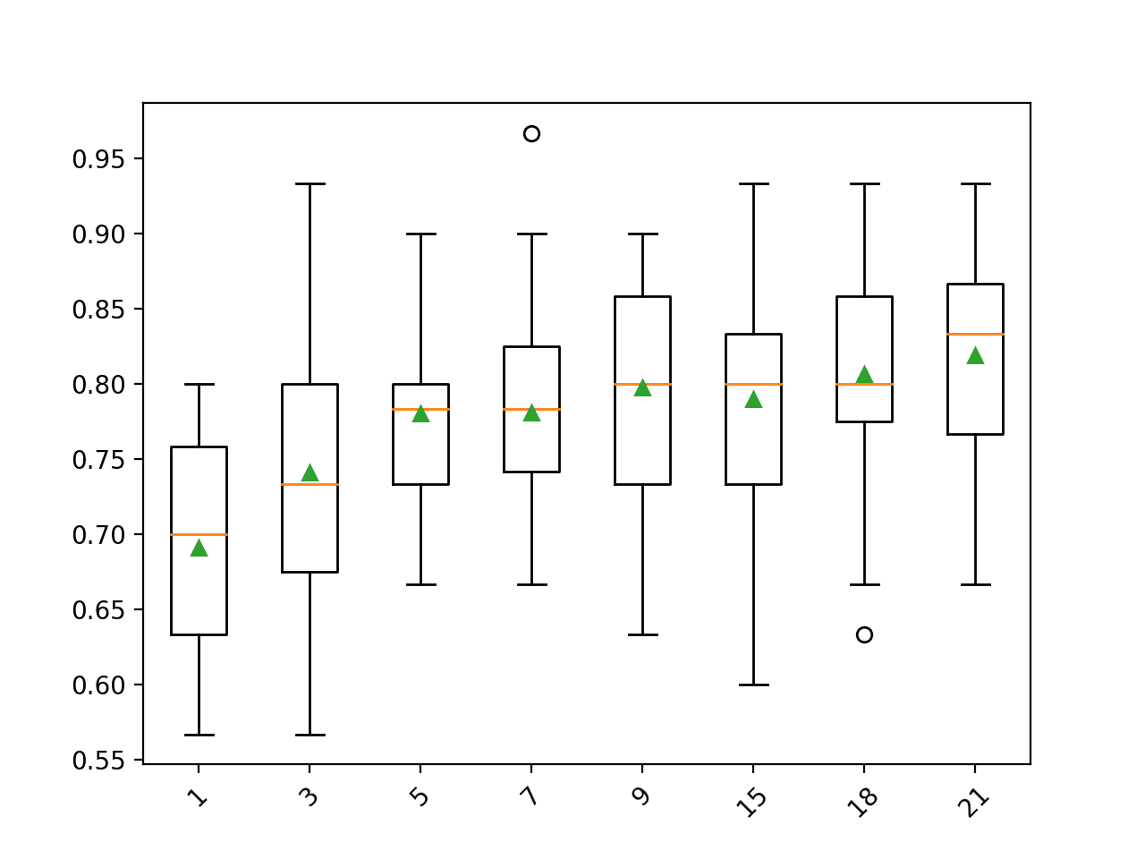
Box and Whisker Plot of Imputation Number of Neighbors for the Horse Colic Dataset
KNNImputer Transform When Making a Prediction
We may wish to create a final modeling pipeline with the nearest neighbor imputation and random forest algorithm, then make a prediction for new data.
This can be achieved by defining the pipeline and fitting it on all available data, then calling the predict() function, passing new data in as an argument.
Importantly, the row of new data must mark any missing values using the NaN value.
...
# define new data
row = [2,1,530101,38.50,66,28,3,3,nan,2,5,4,4,nan,nan,nan,3,5,45.00,8.40,nan,nan,2,2,11300,00000,00000]
The complete example is listed below.
# knn imputation strategy and prediction for the hose colic dataset
from numpy import nan
from pandas import read_csv
from sklearn.ensemble import RandomForestClassifier
from sklearn.impute import KNNImputer
from sklearn.pipeline import Pipeline
# load dataset
url = 'https://raw.githubusercontent.com/jbrownlee/Datasets/master/horse-colic.csv'
dataframe = read_csv(url, header=None, na_values='?')
# split into input and output elements
data = dataframe.values
X, y = data[:, :-1], data[:, -1]
# create the modeling pipeline
pipeline = Pipeline(steps=[('i', KNNImputer(n_neighbors=21)), ('m', RandomForestClassifier())])
# fit the model
pipeline.fit(X, y)
# define new data
row = [2,1,530101,38.50,66,28,3,3,nan,2,5,4,4,nan,nan,nan,3,5,45.00,8.40,nan,nan,2,2,11300,00000,00000]
# make a prediction
yhat = pipeline.predict([row])
# summarize prediction
print('Predicted Class: %d' % yhat[0])
Running the example fits the modeling pipeline on all available data.
A new row of data is defined with missing values marked with NaNs and a classification prediction is made.
Predicted Class: 2
Further Reading
This section provides more resources on the topic if you are looking to go deeper.
Related Tutorials
- Results for Standard Classification and Regression Machine Learning Datasets
- How to Handle Missing Data with Python
Papers
Books
- Applied Predictive Modeling, 2013.
APIs
Dataset
Summary
In this tutorial, you discovered how to use nearest neighbor imputation strategies for missing data in machine learning.
Specifically, you learned:
- Missing values must be marked with NaN values and can be replaced with nearest neighbor estimated values.
- How to load a CSV file with missing values and mark the missing values with NaN values and report the number and percentage of missing values for each column.
- How to impute missing values with nearest neighbor models as a data preparation method when evaluating models and when fitting a final model to make predictions on new data.
Do you have any questions?
Ask your questions in the comments below and I will do my best to answer.
The post kNN Imputation for Missing Values in Machine Learning appeared first on Machine Learning Mastery.