
Author: Jason Brownlee
Many machine learning models perform better when input variables are carefully transformed or scaled prior to modeling.
It is convenient, and therefore common, to apply the same data transforms, such as standardization and normalization, equally to all input variables. This can achieve good results on many problems. Nevertheless, better results may be achieved by carefully selecting which data transform to apply to each input variable prior to modeling.
In this tutorial, you will discover how to apply selective scaling of numerical input variables.
After completing this tutorial, you will know:
- How to load and calculate a baseline predictive performance for the diabetes classification dataset.
- How to evaluate modeling pipelines with data transforms applied blindly to all numerical input variables.
- How to evaluate modeling pipelines with selective normalization and standardization applied to subsets of input variables.
Discover data cleaning, feature selection, data transforms, dimensionality reduction and much more in my new book, with 30 step-by-step tutorials and full Python source code.
Let’s get started.

How to Selectively Scale Numerical Input Variables for Machine Learning
Photo by Marco Verch, some rights reserved.
Tutorial Overview
This tutorial is divided into three parts; they are:
- Diabetes Numerical Dataset
- Non-Selective Scaling of Numerical Inputs
- Normalize All Input Variables
- Standardize All Input Variables
- Selective Scaling of Numerical Inputs
- Normalize Only Non-Gaussian Input Variables
- Standardize Only Gaussian-Like Input Variables
- Selectively Normalize and Standardize Input Variables
Diabetes Numerical Dataset
As the basis of this tutorial, we will use the so-called “diabetes” dataset that has been widely studied as a machine learning dataset since the 1990s.
The dataset classifies patients’ data as either an onset of diabetes within five years or not. There are 768 examples and eight input variables. It is a binary classification problem.
You can learn more about the dataset here:
- Diabetes Dataset (pima-indians-diabetes.csv)
- Diabetes Dataset Description (pima-indians-diabetes.names)
No need to download the dataset; we will download it automatically as part of the worked examples that follow.
Looking at the data, we can see that all nine input variables are numerical.
6,148,72,35,0,33.6,0.627,50,1
1,85,66,29,0,26.6,0.351,31,0
8,183,64,0,0,23.3,0.672,32,1
1,89,66,23,94,28.1,0.167,21,0
0,137,40,35,168,43.1,2.288,33,1
...
We can load this dataset into memory using the Pandas library.
The example below downloads and summarizes the diabetes dataset.
# load and summarize the diabetes dataset
from pandas import read_csv
from pandas.plotting import scatter_matrix
from matplotlib import pyplot
# Load dataset
url = "https://raw.githubusercontent.com/jbrownlee/Datasets/master/pima-indians-diabetes.csv"
dataset = read_csv(url, header=None)
# summarize the shape of the dataset
print(dataset.shape)
# histograms of the variables
dataset.hist()
pyplot.show()
Running the example first downloads the dataset and loads it as a DataFrame.
The shape of the dataset is printed, confirming the number of rows, and nine variables, eight input, and one target.
(768, 9)
Finally, a plot is created showing a histogram for each variable in the dataset.
This is useful as we can see that some variables have a Gaussian or Gaussian-like distribution (1, 2, 5) and others have an exponential-like distribution (0, 3, 4, 6, 7). This may suggest the need for different numerical data transforms for the different types of input variables.
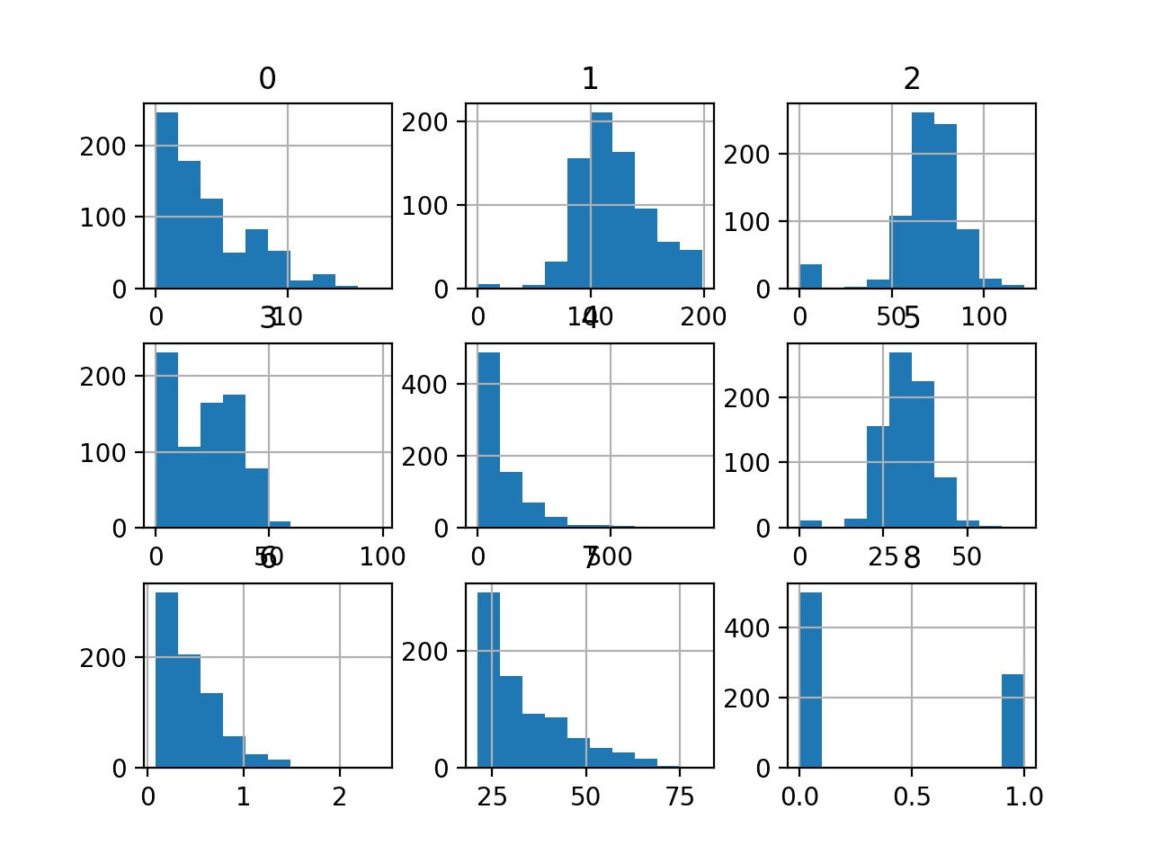
Histogram of Each Variable in the Diabetes Classification Dataset
Now that we are a little familiar with the dataset, let’s try fitting and evaluating a model on the raw dataset.
We will use a logistic regression model as they are a robust and effective linear model for binary classification tasks. We will evaluate the model using repeated stratified k-fold cross-validation, a best practice, and use 10 folds and three repeats.
The complete example is listed below.
# evaluate a logistic regression model on the raw diabetes dataset
from numpy import mean
from numpy import std
from pandas import read_csv
from sklearn.preprocessing import LabelEncoder
from sklearn.model_selection import cross_val_score
from sklearn.model_selection import RepeatedStratifiedKFold
from sklearn.linear_model import LogisticRegression
# load dataset
url = 'https://raw.githubusercontent.com/jbrownlee/Datasets/master/pima-indians-diabetes.csv'
dataframe = read_csv(url, header=None)
data = dataframe.values
# separate into input and output elements
X, y = data[:, :-1], data[:, -1]
# minimally prepare dataset
X = X.astype('float')
y = LabelEncoder().fit_transform(y.astype('str'))
# define the model
model = LogisticRegression(solver='liblinear')
# define the evaluation procedure
cv = RepeatedStratifiedKFold(n_splits=10, n_repeats=3, random_state=1)
# evaluate the model
m_scores = cross_val_score(model, X, y, scoring='accuracy', cv=cv, n_jobs=-1)
# summarize the result
print('Accuracy: %.3f (%.3f)' % (mean(m_scores), std(m_scores)))
Running the example evaluates the model and reports the mean and standard deviation accuracy for fitting a logistic regression model on the raw dataset.
Your specific results may differ given the stochastic nature of the learning algorithm, the stochastic nature of the evaluation procedure, and differences in precision across machines and library versions. Try running the example a few times.
In this case, we can see that the model achieved an accuracy of about 76.8 percent.
Accuracy: 0.768 (0.040)
Now that we have established a baseline in performance on the dataset, let’s see if we can improve the performance using data scaling.
Want to Get Started With Data Preparation?
Take my free 7-day email crash course now (with sample code).
Click to sign-up and also get a free PDF Ebook version of the course.
Non-Selective Scaling of Numerical Inputs
Many algorithms prefer or require that input variables are scaled to a consistent range prior to fitting a model.
This includes the logistic regression model that assumes input variables have a Gaussian probability distribution. It may also provide a more numerically stable model if the input variables are standardized. Nevertheless, even when these expectations are violated, the logistic regression can perform well or best for a given dataset as may be the case for the diabetes dataset.
Two common techniques for scaling numerical input variables are normalization and standardization.
Normalization scales each input variable to the range 0-1 and can be implemented using the MinMaxScaler class in scikit-learn. Standardization scales each input variable to have a mean of 0.0 and a standard deviation of 1.0 and can be implemented using the StandardScaler class in scikit-learn.
To learn more about normalization, standardization, and how to use these methods in scikit-learn, see the tutorial:
A naive approach to data scaling applies a single transform to all input variables, regardless of their scale or probability distribution. And this is often effective.
Let’s try normalizing and standardizing all input variables directly and compare the performance to the baseline logistic regression model fit on the raw data.
Normalize All Input Variables
We can update the baseline code example to use a modeling pipeline where the first step is to apply a scaler and the final step is to fit the model.
This ensures that the scaling operation is fit or prepared on the training set only and then applied to the train and test sets during the cross-validation process, avoiding data leakage. Data leakage can result in an optimistically biased estimate of model performance.
This can be achieved using the Pipeline class where each step in the pipeline is defined as a tuple with a name and the instance of the transform or model to use.
...
# define the modeling pipeline
scaler = MinMaxScaler()
model = LogisticRegression(solver='liblinear')
pipeline = Pipeline([('s',scaler),('m',model)])
Tying this together, the complete example of evaluating a logistic regression on diabetes dataset with all input variables normalized is listed below.
# evaluate a logistic regression model on the normalized diabetes dataset
from numpy import mean
from numpy import std
from pandas import read_csv
from sklearn.preprocessing import LabelEncoder
from sklearn.model_selection import cross_val_score
from sklearn.model_selection import RepeatedStratifiedKFold
from sklearn.pipeline import Pipeline
from sklearn.linear_model import LogisticRegression
from sklearn.preprocessing import MinMaxScaler
# load dataset
url = 'https://raw.githubusercontent.com/jbrownlee/Datasets/master/pima-indians-diabetes.csv'
dataframe = read_csv(url, header=None)
data = dataframe.values
# separate into input and output elements
X, y = data[:, :-1], data[:, -1]
# minimally prepare dataset
X = X.astype('float')
y = LabelEncoder().fit_transform(y.astype('str'))
# define the modeling pipeline
model = LogisticRegression(solver='liblinear')
scaler = MinMaxScaler()
pipeline = Pipeline([('s',scaler),('m',model)])
# define the evaluation procedure
cv = RepeatedStratifiedKFold(n_splits=10, n_repeats=3, random_state=1)
# evaluate the model
m_scores = cross_val_score(pipeline, X, y, scoring='accuracy', cv=cv, n_jobs=-1)
# summarize the result
print('Accuracy: %.3f (%.3f)' % (mean(m_scores), std(m_scores)))
Running the example evaluates the modeling pipeline and reports the mean and standard deviation accuracy for fitting a logistic regression model on the normalized dataset.
Your specific results may differ given the stochastic nature of the learning algorithm, the stochastic nature of the evaluation procedure, and differences in precision across machines and library versions. Try running the example a few times.
In this case, we can see that the normalization of the input variables has resulted in a drop in the mean classification accuracy from 76.8 percent with a model fit on the raw data to about 76.4 percent for the pipeline with normalization.
Accuracy: 0.764 (0.045)
Next, let’s try standardizing all input variables.
Standardize All Input Variables
We can update the modeling pipeline to use standardization instead of normalization for all input variables prior to fitting and evaluating the logistic regression model.
This might be an appropriate transform for those input variables with a Gaussian-like distribution, but perhaps not the other variables.
...
# define the modeling pipeline
scaler = StandardScaler()
model = LogisticRegression(solver='liblinear')
pipeline = Pipeline([('s',scaler),('m',model)])
Tying this together, the complete example of evaluating a logistic regression model on diabetes dataset with all input variables standardized is listed below.
# evaluate a logistic regression model on the standardized diabetes dataset
from numpy import mean
from numpy import std
from pandas import read_csv
from sklearn.preprocessing import LabelEncoder
from sklearn.model_selection import cross_val_score
from sklearn.model_selection import RepeatedStratifiedKFold
from sklearn.pipeline import Pipeline
from sklearn.linear_model import LogisticRegression
from sklearn.preprocessing import StandardScaler
# load dataset
url = 'https://raw.githubusercontent.com/jbrownlee/Datasets/master/pima-indians-diabetes.csv'
dataframe = read_csv(url, header=None)
data = dataframe.values
# separate into input and output elements
X, y = data[:, :-1], data[:, -1]
# minimally prepare dataset
X = X.astype('float')
y = LabelEncoder().fit_transform(y.astype('str'))
# define the modeling pipeline
scaler = StandardScaler()
model = LogisticRegression(solver='liblinear')
pipeline = Pipeline([('s',scaler),('m',model)])
# define the evaluation procedure
cv = RepeatedStratifiedKFold(n_splits=10, n_repeats=3, random_state=1)
# evaluate the model
m_scores = cross_val_score(pipeline, X, y, scoring='accuracy', cv=cv, n_jobs=-1)
# summarize the result
print('Accuracy: %.3f (%.3f)' % (mean(m_scores), std(m_scores)))
Running the example evaluates the modeling pipeline and reports the mean and standard deviation accuracy for fitting a logistic regression model on the standardized dataset.
Your specific results may differ given the stochastic nature of the learning algorithm, the stochastic nature of the evaluation procedure, and differences in precision across machines and library versions. Try running the example a few times.
In this case, we can see that standardizing all numerical input variables has resulted in a lift in mean classification accuracy from 76.8 percent with a model evaluated on the raw dataset to about 77.2 percent for a model evaluated on the dataset with standardized input variables.
Accuracy: 0.772 (0.043)
So far, we have learned that normalizing all variables does not help performance, but standardizing all input variables does help performance.
Next, let’s explore if selectively applying scaling to the input variables can offer further improvement.
Selective Scaling of Numerical Inputs
Data transforms can be applied selectively to input variables using the ColumnTransformer class in scikit-learn.
It allows you to specify the transform (or pipeline of transforms) to apply and the column indexes to apply them to. This can then be used as part of a modeling pipeline and evaluated using cross-validation.
You can learn more about how to use the ColumnTransformer in the tutorial:
We can explore using the ColumnTransformer to selectively apply normalization and standardization to the numerical input variables of the diabetes dataset in order to see if we can achieve further performance improvements.
Normalize Only Non-Gaussian Input Variables
First, let’s try normalizing just those input variables that do not have a Gaussian-like probability distribution and leave the rest of the input variables alone in the raw state.
We can define two groups of input variables using the column indexes, one for the variables with a Gaussian-like distribution, and one for the input variables with the exponential-like distribution.
...
# define column indexes for the variables with "normal" and "exponential" distributions
norm_ix = [1, 2, 5]
exp_ix = [0, 3, 4, 6, 7]
We can then selectively normalize the “exp_ix” group and let the other input variables pass through without any data preparation.
...
# define the selective transforms
t = [('e', MinMaxScaler(), exp_ix)]
selective = ColumnTransformer(transformers=t, remainder='passthrough')
The selective transform can then be used as part of our modeling pipeline.
...
# define the modeling pipeline
model = LogisticRegression(solver='liblinear')
pipeline = Pipeline([('s',selective),('m',model)])
Tying this together, the complete example of evaluating a logistic regression model on data with selective normalization of some input variables is listed below.
# evaluate a logistic regression model on the diabetes dataset with selective normalization
from numpy import mean
from numpy import std
from pandas import read_csv
from sklearn.preprocessing import LabelEncoder
from sklearn.model_selection import cross_val_score
from sklearn.model_selection import RepeatedStratifiedKFold
from sklearn.pipeline import Pipeline
from sklearn.linear_model import LogisticRegression
from sklearn.preprocessing import MinMaxScaler
from sklearn.compose import ColumnTransformer
# load dataset
url = 'https://raw.githubusercontent.com/jbrownlee/Datasets/master/pima-indians-diabetes.csv'
dataframe = read_csv(url, header=None)
data = dataframe.values
# separate into input and output elements
X, y = data[:, :-1], data[:, -1]
# minimally prepare dataset
X = X.astype('float')
y = LabelEncoder().fit_transform(y.astype('str'))
# define column indexes for the variables with "normal" and "exponential" distributions
norm_ix = [1, 2, 5]
exp_ix = [0, 3, 4, 6, 7]
# define the selective transforms
t = [('e', MinMaxScaler(), exp_ix)]
selective = ColumnTransformer(transformers=t, remainder='passthrough')
# define the modeling pipeline
model = LogisticRegression(solver='liblinear')
pipeline = Pipeline([('s',selective),('m',model)])
# define the evaluation procedure
cv = RepeatedStratifiedKFold(n_splits=10, n_repeats=3, random_state=1)
# evaluate the model
m_scores = cross_val_score(pipeline, X, y, scoring='accuracy', cv=cv, n_jobs=-1)
# summarize the result
print('Accuracy: %.3f (%.3f)' % (mean(m_scores), std(m_scores)))
Running the example evaluates the modeling pipeline and reports the mean and standard deviation accuracy.
Your specific results may differ given the stochastic nature of the learning algorithm, the stochastic nature of the evaluation procedure, and differences in precision across machines and library versions. Try running the example a few times.
In this case, we can see slightly better performance, increasing mean accuracy with the baseline model fit on the raw dataset with 76.8 percent to about 76.9 with selective normalization of some input variables.
The results are not as good as standardizing all input variables though.
Accuracy: 0.769 (0.043)
Standardize Only Gaussian-Like Input Variables
We can repeat the experiment from the previous section, although in this case, selectively standardize those input variables that have a Gaussian-like distribution and leave the remaining input variables untouched.
...
# define the selective transforms
t = [('n', StandardScaler(), norm_ix)]
selective = ColumnTransformer(transformers=t, remainder='passthrough')
Tying this together, the complete example of evaluating a logistic regression model on data with selective standardizing of some input variables is listed below.
# evaluate a logistic regression model on the diabetes dataset with selective standardization
from numpy import mean
from numpy import std
from pandas import read_csv
from sklearn.preprocessing import LabelEncoder
from sklearn.model_selection import cross_val_score
from sklearn.model_selection import RepeatedStratifiedKFold
from sklearn.pipeline import Pipeline
from sklearn.linear_model import LogisticRegression
from sklearn.preprocessing import StandardScaler
from sklearn.compose import ColumnTransformer
# load dataset
url = 'https://raw.githubusercontent.com/jbrownlee/Datasets/master/pima-indians-diabetes.csv'
dataframe = read_csv(url, header=None)
data = dataframe.values
# separate into input and output elements
X, y = data[:, :-1], data[:, -1]
# minimally prepare dataset
X = X.astype('float')
y = LabelEncoder().fit_transform(y.astype('str'))
# define column indexes for the variables with "normal" and "exponential" distributions
norm_ix = [1, 2, 5]
exp_ix = [0, 3, 4, 6, 7]
# define the selective transforms
t = [('n', StandardScaler(), norm_ix)]
selective = ColumnTransformer(transformers=t, remainder='passthrough')
# define the modeling pipeline
model = LogisticRegression(solver='liblinear')
pipeline = Pipeline([('s',selective),('m',model)])
# define the evaluation procedure
cv = RepeatedStratifiedKFold(n_splits=10, n_repeats=3, random_state=1)
# evaluate the model
m_scores = cross_val_score(pipeline, X, y, scoring='accuracy', cv=cv, n_jobs=-1)
# summarize the result
print('Accuracy: %.3f (%.3f)' % (mean(m_scores), std(m_scores)))
Running the example evaluates the modeling pipeline and reports the mean and standard deviation accuracy.
Your specific results may differ given the stochastic nature of the learning algorithm, the stochastic nature of the evaluation procedure, and differences in precision across machines and library versions. Try running the example a few times.
In this case, we can see that we achieved a lift in performance over both the baseline model fit on the raw dataset with 76.8 percent and over the standardization of all input variables that achieved 77.2 percent. With selective standardization, we have achieved a mean accuracy of about 77.3 percent, a modest but measurable bump.
Accuracy: 0.773 (0.041)
Selectively Normalize and Standardize Input Variables
The results so far raise the question as to whether we can get a further lift by combining the use of selective normalization and standardization on the dataset at the same time.
This can be achieved by defining both transforms and their respective column indexes for the ColumnTransformer class, with no remaining variables being passed through.
...
# define the selective transforms
t = [('e', MinMaxScaler(), exp_ix), ('n', StandardScaler(), norm_ix)]
selective = ColumnTransformer(transformers=t)
Tying this together, the complete example of evaluating a logistic regression model on data with selective normalization and standardization of the input variables is listed below.
# evaluate a logistic regression model on the diabetes dataset with selective scaling
from numpy import mean
from numpy import std
from pandas import read_csv
from sklearn.preprocessing import LabelEncoder
from sklearn.model_selection import cross_val_score
from sklearn.model_selection import RepeatedStratifiedKFold
from sklearn.pipeline import Pipeline
from sklearn.linear_model import LogisticRegression
from sklearn.preprocessing import MinMaxScaler
from sklearn.preprocessing import StandardScaler
from sklearn.compose import ColumnTransformer
# load dataset
url = 'https://raw.githubusercontent.com/jbrownlee/Datasets/master/pima-indians-diabetes.csv'
dataframe = read_csv(url, header=None)
data = dataframe.values
# separate into input and output elements
X, y = data[:, :-1], data[:, -1]
# minimally prepare dataset
X = X.astype('float')
y = LabelEncoder().fit_transform(y.astype('str'))
# define column indexes for the variables with "normal" and "exponential" distributions
norm_ix = [1, 2, 5]
exp_ix = [0, 3, 4, 6, 7]
# define the selective transforms
t = [('e', MinMaxScaler(), exp_ix), ('n', StandardScaler(), norm_ix)]
selective = ColumnTransformer(transformers=t)
# define the modeling pipeline
model = LogisticRegression(solver='liblinear')
pipeline = Pipeline([('s',selective),('m',model)])
# define the evaluation procedure
cv = RepeatedStratifiedKFold(n_splits=10, n_repeats=3, random_state=1)
# evaluate the model
m_scores = cross_val_score(pipeline, X, y, scoring='accuracy', cv=cv, n_jobs=-1)
# summarize the result
print('Accuracy: %.3f (%.3f)' % (mean(m_scores), std(m_scores)))
Running the example evaluates the modeling pipeline and reports the mean and standard deviation accuracy.
Your specific results may differ given the stochastic nature of the learning algorithm, the stochastic nature of the evaluation procedure, and differences in precision across machines and library versions. Try running the example a few times.
In this case, interestingly, we can see that we have achieved the same performance as standardizing all input variables with 77.2 percent.
Further, the results suggest that the chosen model performs better when the non-Gaussian like variables are left as-is than being standardized or normalized.
I would not have guessed at this finding, which highlights the importance of careful experimentation.
Accuracy: 0.772 (0.040)
Can you do better?
Try other transforms or combinations of transforms and see if you can achieve better results.
Share your findings in the comments below.
Further Reading
This section provides more resources on the topic if you are looking to go deeper.
Tutorials
- Best Results for Standard Machine Learning Datasets
- How to Use the ColumnTransformer for Data Preparation
- How to Use StandardScaler and MinMaxScaler Transforms in Python
APIs
Summary
In this tutorial, you discovered how to apply selective scaling of numerical input variables.
Specifically, you learned:
- How to load and calculate a baseline predictive performance for the diabetes classification dataset.
- How to evaluate modeling pipelines with data transforms applied blindly to all numerical input variables.
- How to evaluate modeling pipelines with selective normalization and standardization applied to subsets of input variables.
Do you have any questions?
Ask your questions in the comments below and I will do my best to answer.
The post How to Selectively Scale Numerical Input Variables for Machine Learning appeared first on Machine Learning Mastery.