How to Configure k-Fold Cross-Validation

Author: Jason Brownlee

The k-fold cross-validation procedure is a standard method for estimating the performance of a machine learning algorithm on a dataset.

A common value for k is 10, although how do we know that this configuration is appropriate for our dataset and our algorithms?

One approach is to explore the effect of different k values on the estimate of model performance and compare this to an ideal test condition. This can help to choose an appropriate value for k.

Once a k-value is chosen, it can be used to evaluate a suite of different algorithms on the dataset and the distribution of results can be compared to an evaluation of the same algorithms using an ideal test condition to see if they are highly correlated or not. If correlated, it confirms the chosen configuration is a robust approximation for the ideal test condition.

In this tutorial, you will discover how to configure and evaluate configurations of k-fold cross-validation.

After completing this tutorial, you will know:

How to evaluate a machine learning algorithm using k-fold cross-validation on a dataset.
How to perform a sensitivity analysis of k-values for k-fold cross-validation.
How to calculate the correlation between a cross-validation test harness and an ideal test condition.

Let’s get started.

How to Configure k-Fold Cross-Validation
Photo by Patricia Farrell, some rights reserved.

Tutorial Overview

This tutorial is divided into three parts; they are:

k-Fold Cross-Validation
Sensitivity Analysis for k
Correlation of Test Harness With Target

k-Fold Cross-Validation

It is common to evaluate machine learning models on a dataset using k-fold cross-validation.

The k-fold cross-validation procedure divides a limited dataset into k non-overlapping folds. Each of the k folds is given an opportunity to be used as a held-back test set, whilst all other folds collectively are used as a training dataset. A total of k models are fit and evaluated on the k hold-out test sets and the mean performance is reported.

For more on the k-fold cross-validation procedure, see the tutorial:

A Gentle Introduction to k-fold Cross-Validation

The k-fold cross-validation procedure can be implemented easily using the scikit-learn machine learning library.

First, let’s define a synthetic classification dataset that we can use as the basis of this tutorial.

The make_classification() function can be used to create a synthetic binary classification dataset. We will configure it to generate 100 samples each with 20 input features, 15 of which contribute to the target variable.

The example below creates and summarizes the dataset.

# test classification dataset
from sklearn.datasets import make_classification
# define dataset
X, y = make_classification(n_samples=100, n_features=20, n_informative=15, n_redundant=5, random_state=1)
# summarize the dataset
print(X.shape, y.shape)

Running the example creates the dataset and confirms that it contains 100 samples and 10 input variables.

The fixed seed for the pseudorandom number generator ensures that we get the same samples each time the dataset is generated.

(100, 20) (100,)

Next, we can evaluate a model on this dataset using k-fold cross-validation.

We will evaluate a LogisticRegression model and use the KFold class to perform the cross-validation, configured to shuffle the dataset and set k=10, a popular default.

The cross_val_score() function will be used to perform the evaluation, taking the dataset and cross-validation configuration and returning a list of scores calculated for each fold.

The complete example is listed below.

# evaluate a logistic regression model using k-fold cross-validation
from numpy import mean
from numpy import std
from sklearn.datasets import make_classification
from sklearn.model_selection import KFold
from sklearn.model_selection import cross_val_score
from sklearn.linear_model import LogisticRegression
# create dataset
X, y = make_classification(n_samples=100, n_features=20, n_informative=15, n_redundant=5, random_state=1)
# prepare the cross-validation procedure
cv = KFold(n_splits=10, random_state=1, shuffle=True)
# create model
model = LogisticRegression()
# evaluate model
scores = cross_val_score(model, X, y, scoring='accuracy', cv=cv, n_jobs=-1)
# report performance
print('Accuracy: %.3f (%.3f)' % (mean(scores), std(scores)))

Running the example creates the dataset, then evaluates a logistic regression model on it using 10-fold cross-validation. The mean classification accuracy on the dataset is then reported.

Your specific results may vary given the stochastic nature of the learning algorithm. Try running the example a few times.

In this case, we can see that the model achieved an estimated classification accuracy of about 85.0 percent.

Accuracy: 0.850 (0.128)

Now that we are familiar with k-fold cross-validation, let’s look at how we might configure the procedure.

Sensitivity Analysis for k

The key configuration parameter for k-fold cross-validation is k that defines the number folds in which to split a given dataset.

Common values are k=3, k=5, and k=10, and by far the most popular value used in applied machine learning to evaluate models is k=10. The reason for this is studies were performed and k=10 was found to provide good trade-off of low computational cost and low bias in an estimate of model performance.

How do we know what value of k to use when evaluating models on our own dataset?

You can choose k=10, but how do you know this makes sense for your dataset?

One approach to answering this question is to perform a sensitivity analysis for different k values. That is, evaluate the performance of the same model on the same dataset with different values of k and see how they compare.

The expectation is that low values of k will result in a noisy estimate of model performance and large values of k will result in a less noisy estimate of model performance.

But noisy compared to what?

We don’t know the true performance of the model when making predictions on new/unseen data, as we don’t have access to new/unseen data. If we did, we would make use of it in the evaluation of the model.

Nevertheless, we can choose a test condition that represents an “ideal” or as-best-as-we-can-achieve “ideal” estimate of model performance.

One approach would be to train the model on all available data and estimate the performance on a separate large and representative hold-out dataset. The performance on this hold-out dataset would represent the “true” performance of the model and any cross-validation performances on the training dataset would represent an estimate of this score.

This is rarely possible as we often do not have enough data to hold some back and use it as a test set. Kaggle machine learning competitions are one exception to this, where we do have a hold-out test set, a sample of which is evaluated via submissions.

Instead, we can simulate this case using the leave-one-out cross-validation (LOOCV), a computationally expensive version of cross-validation where k=N, and N is the total number of examples in the training dataset. That is, each sample in the training set is given an example to be used alone as the test evaluation dataset. It is rarely used for large datasets as it is computationally expensive, although it can provide a good estimate of model performance given the available data.

We can then compare the mean classification accuracy for different k values to the mean classification accuracy from LOOCV on the same dataset. The difference between the scores provides a rough proxy for how well a k value approximates the ideal model evaluation test condition.

Let’s explore how to implement a sensitivity analysis of k-fold cross-validation.

First, let’s define a function to create the dataset. This allows you to change the dataset to your own if you desire.

# create the dataset
def get_dataset(n_samples=100):
	X, y = make_classification(n_samples=n_samples, n_features=20, n_informative=15, n_redundant=5, random_state=1)
	return X, y

Next, we can define a dataset to create the model to evaluate.

Again, this separation allows you to change the model to your own if you desire.

# retrieve the model to be evaluate
def get_model():
	model = LogisticRegression()
	return model

Next, you can define a function to evaluate the model on the dataset given a test condition. The test condition could be an instance of the KFold configured with a given k-value, or it could be an instance of LeaveOneOut that represents our ideal test condition.

The function returns the mean classification accuracy as well as the min and max accuracy from the folds. We can use the min and max to summarize the distribution of scores.

# evaluate the model using a given test condition
def evaluate_model(cv):
	# get the dataset
	X, y = get_dataset()
	# get the model
	model = get_model()
	# evaluate the model
	scores = cross_val_score(model, X, y, scoring='accuracy', cv=cv, n_jobs=-1)
	# return scores
	return mean(scores), scores.min(), scores.max()

Next, we can calculate the model performance using the LOOCV procedure.

...
# calculate the ideal test condition
ideal, _, _ = evaluate_model(LeaveOneOut())
print('Ideal: %.3f' % ideal)

We can then define the k values to evaluate. In this case, we will test values between 2 and 30.

...
# define folds to test
folds = range(2,31)

We can then evaluate each value in turn and store the results as we go.

...
# record mean and min/max of each set of results
means, mins, maxs = list(),list(),list()
# evaluate each k value
for k in folds:
	# define the test condition
	cv = KFold(n_splits=k, shuffle=True, random_state=1)
	# evaluate k value
	k_mean, k_min, k_max = evaluate_model(cv)
	# report performance
	print('> folds=%d, accuracy=%.3f (%.3f,%.3f)' % (k, k_mean, k_min, k_max))
	# store mean accuracy
	means.append(k_mean)
	# store min and max relative to the mean
	mins.append(k_mean - k_min)
	maxs.append(k_max - k_mean)

Finally, we can plot the results for interpretation.

...
# line plot of k mean values with min/max error bars
pyplot.errorbar(folds, means, yerr=[mins, maxs], fmt='o')
# plot the ideal case in a separate color
pyplot.plot(folds, [ideal for _ in range(len(folds))], color='r')
# show the plot
pyplot.show()

Tying this together, the complete example is listed below.

# sensitivity analysis of k in k-fold cross-validation
from numpy import mean
from sklearn.datasets import make_classification
from sklearn.model_selection import LeaveOneOut
from sklearn.model_selection import KFold
from sklearn.model_selection import cross_val_score
from sklearn.linear_model import LogisticRegression
from matplotlib import pyplot

# create the dataset
def get_dataset(n_samples=100):
	X, y = make_classification(n_samples=n_samples, n_features=20, n_informative=15, n_redundant=5, random_state=1)
	return X, y

# retrieve the model to be evaluate
def get_model():
	model = LogisticRegression()
	return model

# evaluate the model using a given test condition
def evaluate_model(cv):
	# get the dataset
	X, y = get_dataset()
	# get the model
	model = get_model()
	# evaluate the model
	scores = cross_val_score(model, X, y, scoring='accuracy', cv=cv, n_jobs=-1)
	# return scores
	return mean(scores), scores.min(), scores.max()

# calculate the ideal test condition
ideal, _, _ = evaluate_model(LeaveOneOut())
print('Ideal: %.3f' % ideal)
# define folds to test
folds = range(2,31)
# record mean and min/max of each set of results
means, mins, maxs = list(),list(),list()
# evaluate each k value
for k in folds:
	# define the test condition
	cv = KFold(n_splits=k, shuffle=True, random_state=1)
	# evaluate k value
	k_mean, k_min, k_max = evaluate_model(cv)
	# report performance
	print('> folds=%d, accuracy=%.3f (%.3f,%.3f)' % (k, k_mean, k_min, k_max))
	# store mean accuracy
	means.append(k_mean)
	# store min and max relative to the mean
	mins.append(k_mean - k_min)
	maxs.append(k_max - k_mean)
# line plot of k mean values with min/max error bars
pyplot.errorbar(folds, means, yerr=[mins, maxs], fmt='o')
# plot the ideal case in a separate color
pyplot.plot(folds, [ideal for _ in range(len(folds))], color='r')
# show the plot
pyplot.show()

Running the example first reports the LOOCV, then the mean, min, and max accuracy for each k value that was evaluated.

Your specific results may vary given the stochastic nature of the learning algorithm. Try running the example a few times.

In this case, we can see that the LOOCV result was about 84 percent, slightly lower than the k=10 result of 85 percent.

Ideal: 0.840
> folds=2, accuracy=0.740 (0.700,0.780)
> folds=3, accuracy=0.749 (0.697,0.824)
> folds=4, accuracy=0.790 (0.640,0.920)
> folds=5, accuracy=0.810 (0.600,0.950)
> folds=6, accuracy=0.820 (0.688,0.941)
> folds=7, accuracy=0.799 (0.571,1.000)
> folds=8, accuracy=0.811 (0.385,0.923)
> folds=9, accuracy=0.829 (0.636,1.000)
> folds=10, accuracy=0.850 (0.600,1.000)
> folds=11, accuracy=0.829 (0.667,1.000)
> folds=12, accuracy=0.785 (0.250,1.000)
> folds=13, accuracy=0.839 (0.571,1.000)
> folds=14, accuracy=0.807 (0.429,1.000)
> folds=15, accuracy=0.821 (0.571,1.000)
> folds=16, accuracy=0.827 (0.500,1.000)
> folds=17, accuracy=0.816 (0.600,1.000)
> folds=18, accuracy=0.831 (0.600,1.000)
> folds=19, accuracy=0.826 (0.600,1.000)
> folds=20, accuracy=0.830 (0.600,1.000)
> folds=21, accuracy=0.814 (0.500,1.000)
> folds=22, accuracy=0.820 (0.500,1.000)
> folds=23, accuracy=0.802 (0.250,1.000)
> folds=24, accuracy=0.804 (0.250,1.000)
> folds=25, accuracy=0.810 (0.250,1.000)
> folds=26, accuracy=0.804 (0.250,1.000)
> folds=27, accuracy=0.818 (0.250,1.000)
> folds=28, accuracy=0.821 (0.250,1.000)
> folds=29, accuracy=0.822 (0.250,1.000)
> folds=30, accuracy=0.822 (0.333,1.000)

A line plot is created comparing the mean accuracy scores to the LOOCV result with the min and max of each result distribution indicated using error bars.

The results suggest that for this model on this dataset, most k values underestimate the performance of the model compared to the ideal case. The results suggest that perhaps k=10 alone is slightly optimistic and perhaps k=13 might be a more accurate estimate.

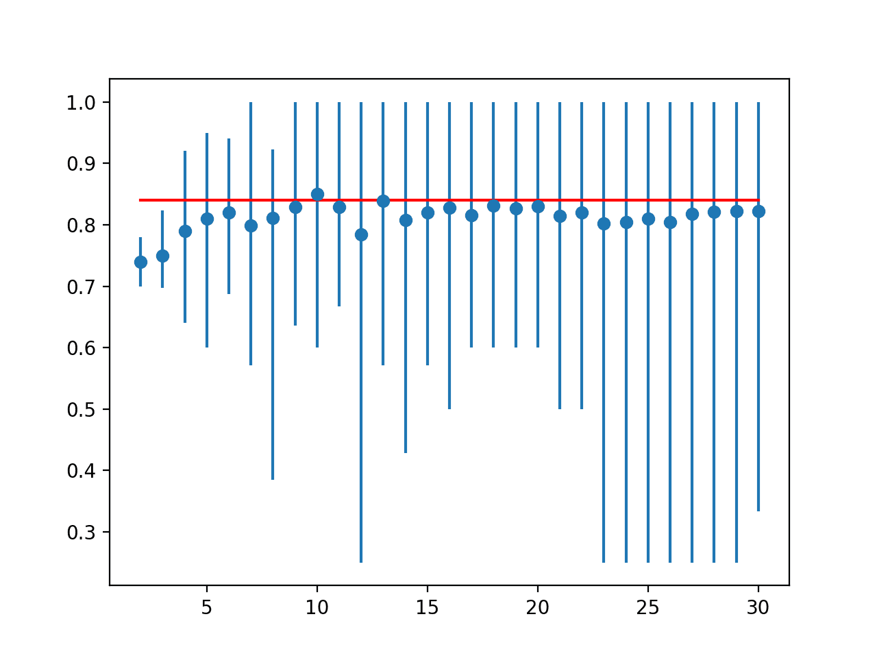
Line Plot of Mean Accuracy for Cross-Validation k-Values With Error Bars (Blue) vs. the Ideal Case (red)

This provides a template that you can use to perform a sensitivity analysis of k values of your chosen model on your dataset against a given ideal test condition.

Correlation of Test Harness With Target

Once a test harness is chosen, another consideration is how well it matches the ideal test condition across different algorithms.

It is possible that for some algorithms and some configurations, the k-fold cross-validation will be a better approximation of the ideal test condition compared to other algorithms and algorithm configurations.

We can evaluate and report on this relationship explicitly. This can be achieved by calculating how well the k-fold cross-validation results across a range of algorithms match the evaluation of the same algorithms on the ideal test condition.

The Pearson’s correlation coefficient can be calculated between the two groups of scores to measure how closely they match. That is, do they change together in the same ways: when one algorithm looks better than another via k-fold cross-validation, does this hold on the ideal test condition?

We expect to see a strong positive correlation between the scores, such as 0.5 or higher. A low correlation suggests the need to change the k-fold cross-validation test harness to better match the ideal test condition.

First, we can define a function that will create a list of standard machine learning models to evaluate via each test harness.

# get a list of models to evaluate
def get_models():
	models = list()
	models.append(LogisticRegression())
	models.append(RidgeClassifier())
	models.append(SGDClassifier())
	models.append(PassiveAggressiveClassifier())
	models.append(KNeighborsClassifier())
	models.append(DecisionTreeClassifier())
	models.append(ExtraTreeClassifier())
	models.append(LinearSVC())
	models.append(SVC())
	models.append(GaussianNB())
	models.append(AdaBoostClassifier())
	models.append(BaggingClassifier())
	models.append(RandomForestClassifier())
	models.append(ExtraTreesClassifier())
	models.append(GaussianProcessClassifier())
	models.append(GradientBoostingClassifier())
	models.append(LinearDiscriminantAnalysis())
	models.append(QuadraticDiscriminantAnalysis())
	return models

We will use k=10 for the chosen test harness.

We can then enumerate each model and evaluate it using 10-fold cross-validation and our ideal test condition, in this case, LOOCV.

...
# define test conditions
ideal_cv = LeaveOneOut()
cv = KFold(n_splits=10, shuffle=True, random_state=1)
# get the list of models to consider
models = get_models()
# collect results
ideal_results, cv_results = list(), list()
# evaluate each model
for model in models:
	# evaluate model using each test condition
	cv_mean = evaluate_model(cv, model)
	ideal_mean = evaluate_model(ideal_cv, model)
	# check for invalid results
	if isnan(cv_mean) or isnan(ideal_mean):
		continue
	# store results
	cv_results.append(cv_mean)
	ideal_results.append(ideal_mean)
	# summarize progress
	print('>%s: ideal=%.3f, cv=%.3f' % (type(model).__name__, ideal_mean, cv_mean))

We can then calculate the correlation between the mean classification accuracy from the 10-fold cross-validation test harness and the LOOCV test harness.

...
# calculate the correlation between each test condition
corr, _ = pearsonr(cv_results, ideal_results)
print('Correlation: %.3f' % corr)

Finally, we can create a scatter plot of the two sets of results and draw a line of best fit to visually see how well they change together.

...
# scatter plot of results
pyplot.scatter(cv_results, ideal_results)
# plot the line of best fit
coeff, bias = polyfit(cv_results, ideal_results, 1)
line = coeff * asarray(cv_results) + bias
pyplot.plot(cv_results, line, color='r')
# show the plot
pyplot.show()

Tying all of this together, the complete example is listed below.

# correlation between test harness and ideal test condition
from numpy import mean
from numpy import isnan
from numpy import asarray
from numpy import polyfit
from scipy.stats import pearsonr
from matplotlib import pyplot
from sklearn.datasets import make_classification
from sklearn.model_selection import KFold
from sklearn.model_selection import LeaveOneOut
from sklearn.model_selection import cross_val_score
from sklearn.linear_model import LogisticRegression
from sklearn.linear_model import RidgeClassifier
from sklearn.linear_model import SGDClassifier
from sklearn.linear_model import PassiveAggressiveClassifier
from sklearn.neighbors import KNeighborsClassifier
from sklearn.tree import DecisionTreeClassifier
from sklearn.tree import ExtraTreeClassifier
from sklearn.svm import LinearSVC
from sklearn.svm import SVC
from sklearn.naive_bayes import GaussianNB
from sklearn.ensemble import AdaBoostClassifier
from sklearn.ensemble import BaggingClassifier
from sklearn.ensemble import RandomForestClassifier
from sklearn.ensemble import ExtraTreesClassifier
from sklearn.gaussian_process import GaussianProcessClassifier
from sklearn.ensemble import GradientBoostingClassifier
from sklearn.discriminant_analysis import LinearDiscriminantAnalysis
from sklearn.discriminant_analysis import QuadraticDiscriminantAnalysis

# create the dataset
def get_dataset(n_samples=100):
	X, y = make_classification(n_samples=n_samples, n_features=20, n_informative=15, n_redundant=5, random_state=1)
	return X, y

# get a list of models to evaluate
def get_models():
	models = list()
	models.append(LogisticRegression())
	models.append(RidgeClassifier())
	models.append(SGDClassifier())
	models.append(PassiveAggressiveClassifier())
	models.append(KNeighborsClassifier())
	models.append(DecisionTreeClassifier())
	models.append(ExtraTreeClassifier())
	models.append(LinearSVC())
	models.append(SVC())
	models.append(GaussianNB())
	models.append(AdaBoostClassifier())
	models.append(BaggingClassifier())
	models.append(RandomForestClassifier())
	models.append(ExtraTreesClassifier())
	models.append(GaussianProcessClassifier())
	models.append(GradientBoostingClassifier())
	models.append(LinearDiscriminantAnalysis())
	models.append(QuadraticDiscriminantAnalysis())
	return models

# evaluate the model using a given test condition
def evaluate_model(cv, model):
	# get the dataset
	X, y = get_dataset()
	# evaluate the model
	scores = cross_val_score(model, X, y, scoring='accuracy', cv=cv, n_jobs=-1)
	# return scores
	return mean(scores)

# define test conditions
ideal_cv = LeaveOneOut()
cv = KFold(n_splits=10, shuffle=True, random_state=1)
# get the list of models to consider
models = get_models()
# collect results
ideal_results, cv_results = list(), list()
# evaluate each model
for model in models:
	# evaluate model using each test condition
	cv_mean = evaluate_model(cv, model)
	ideal_mean = evaluate_model(ideal_cv, model)
	# check for invalid results
	if isnan(cv_mean) or isnan(ideal_mean):
		continue
	# store results
	cv_results.append(cv_mean)
	ideal_results.append(ideal_mean)
	# summarize progress
	print('>%s: ideal=%.3f, cv=%.3f' % (type(model).__name__, ideal_mean, cv_mean))
# calculate the correlation between each test condition
corr, _ = pearsonr(cv_results, ideal_results)
print('Correlation: %.3f' % corr)
# scatter plot of results
pyplot.scatter(cv_results, ideal_results)
# plot the line of best fit
coeff, bias = polyfit(cv_results, ideal_results, 1)
line = coeff * asarray(cv_results) + bias
pyplot.plot(cv_results, line, color='r')
# label the plot
pyplot.title('10-fold CV vs LOOCV Mean Accuracy')
pyplot.xlabel('Mean Accuracy (10-fold CV)')
pyplot.ylabel('Mean Accuracy (LOOCV)')
# show the plot
pyplot.show()

Running the example reports the mean classification accuracy for each algorithm calculated via each test harness.

Your specific results may vary given the stochastic nature of the learning algorithm. Try running the example a few times.

You may see some warnings that you can safely ignore, such as:

Variables are collinear

We can see that for some algorithms, the test harness over-estimates the accuracy compared to LOOCV, and in other cases, it under-estimates the accuracy. This is to be expected.

At the end of the run, we can see that the correlation between the two sets of results is reported. In this case, we can see that a correlation of 0.746 is reported, which is a good strong positive correlation. The results suggest that 10-fold cross-validation does provide a good approximation for the LOOCV test harness on this dataset as calculated with 18 popular machine learning algorithms.

>LogisticRegression: ideal=0.840, cv=0.850
>RidgeClassifier: ideal=0.830, cv=0.830
>SGDClassifier: ideal=0.730, cv=0.790
>PassiveAggressiveClassifier: ideal=0.780, cv=0.760
>KNeighborsClassifier: ideal=0.760, cv=0.770
>DecisionTreeClassifier: ideal=0.690, cv=0.630
>ExtraTreeClassifier: ideal=0.710, cv=0.620
>LinearSVC: ideal=0.850, cv=0.830
>SVC: ideal=0.900, cv=0.880
>GaussianNB: ideal=0.730, cv=0.720
>AdaBoostClassifier: ideal=0.740, cv=0.740
>BaggingClassifier: ideal=0.770, cv=0.740
>RandomForestClassifier: ideal=0.810, cv=0.790
>ExtraTreesClassifier: ideal=0.820, cv=0.820
>GaussianProcessClassifier: ideal=0.790, cv=0.760
>GradientBoostingClassifier: ideal=0.820, cv=0.820
>LinearDiscriminantAnalysis: ideal=0.830, cv=0.830
>QuadraticDiscriminantAnalysis: ideal=0.610, cv=0.760
Correlation: 0.746

Finally, a scatter plot is created comparing the distribution of mean accuracy scores for the test harness (x-axis) vs. the accuracy scores via LOOCV (y-axis).

A red line of best fit is drawn through the results showing the strong linear correlation.

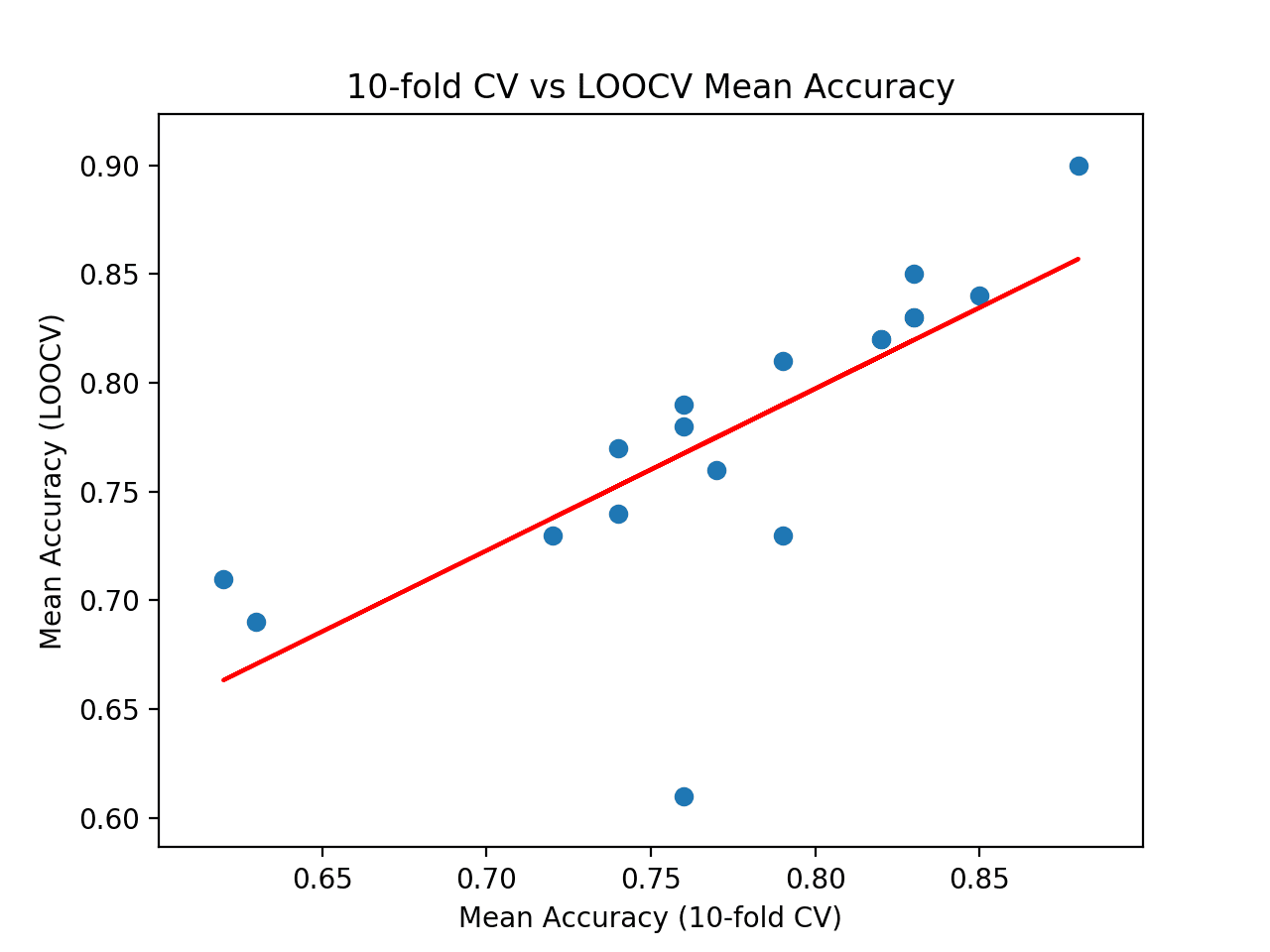
Scatter Plot of Cross-Validation vs. Ideal Test Mean Accuracy With Line of Best Fit

This provides a harness for comparing your chosen test harness to an ideal test condition on your own dataset.

Summary

In this tutorial, you discovered how to configure and evaluate configurations of k-fold cross-validation.

Specifically, you learned:

How to evaluate a machine learning algorithm using k-fold cross-validation on a dataset.
How to perform a sensitivity analysis of k-values for k-fold cross-validation.
How to calculate the correlation between a cross-validation test harness and an ideal test condition.

Do you have any questions?
Ask your questions in the comments below and I will do my best to answer.

The post How to Configure k-Fold Cross-Validation appeared first on Machine Learning Mastery.

Go to Source

How to Configure k-Fold Cross-Validation

Tutorial Overview

k-Fold Cross-Validation

Sensitivity Analysis for k

Correlation of Test Harness With Target

Further Reading

Tutorials

APIs

Articles

Summary