
Author: Jason Brownlee
Computational learning theory, or statistical learning theory, refers to mathematical frameworks for quantifying learning tasks and algorithms.
These are sub-fields of machine learning that a machine learning practitioner does not need to know in great depth in order to achieve good results on a wide range of problems. Nevertheless, it is a sub-field where having a high-level understanding of some of the more prominent methods may provide insight into the broader task of learning from data.
In this post, you will discover a gentle introduction to computational learning theory for machine learning.
After reading this post, you will know:
- Computational learning theory uses formal methods to study learning tasks and learning algorithms.
- PAC learning provides a way to quantify the computational difficulty of a machine learning task.
- VC Dimension provides a way to quantify the computational capacity of a machine learning algorithm.
Let’s get started.

A Gentle Introduction to Computational Learning Theory
Photo by someone10x, some rights reserved.
Tutorial Overview
This tutorial is divided into three parts; they are:
- Computational Learning Theory
- PAC Learning (Theory of Learning Problems)
- VC Dimension (Theory of Learning Algorithms)
Computational Learning Theory
Computational learning theory, or CoLT for short, is a field of study concerned with the use of formal mathematical methods applied to learning systems.
It seeks to use the tools of theoretical computer science to quantify learning problems. This includes characterizing the difficulty of learning specific tasks.
Computational learning theory may be thought of as an extension or sibling of statistical learning theory, or SLT for short, that uses formal methods to quantify learning algorithms.
- Computational Learning Theory (CoLT): Formal study of learning tasks.
- Statistical Learning Theory (SLT): Formal study of learning algorithms.
This division of learning tasks vs. learning algorithms is arbitrary, and in practice, there is a lot of overlap between the two fields.
One can extend statistical learning theory by taking computational complexity of the learner into account. This field is called computational learning theory or COLT.
— Page 210, Machine Learning: A Probabilistic Perspective, 2012.
They might be considered synonyms in modern usage.
… a theoretical framework known as computational learning theory, also some- times called statistical learning theory.
— Page 344, Pattern Recognition and Machine Learning, 2006.
The focus in computational learning theory is typically on supervised learning tasks. Formal analysis of real problems and real algorithms is very challenging. As such, it is common to reduce the complexity of the analysis by focusing on binary classification tasks and even simple binary rule-based systems. As such, the practical application of the theorems may be limited or challenging to interpret for real problems and algorithms.
The main unanswered question in learning is this: How can we be sure that our learning algorithm has produced a hypothesis that will predict the correct value for previously unseen inputs?
— Page 713, Artificial Intelligence: A Modern Approach, 3rd edition, 2009.
Questions explored in computational learning theory might include:
- How do we know a model has a good approximation for the target function?
- What hypothesis space should be used?
- How do we know if we have a local or globally good solution?
- How do we avoid overfitting?
- How many data examples are needed?
As a machine learning practitioner, it can be useful to know about computational learning theory and some of the main areas of investigation. The field provides a useful grounding for what we are trying to achieve when fitting models on data, and it may provide insight into the methods.
There are many subfields of study, although perhaps two of the most widely discussed areas of study from computational learning theory are:
- PAC Learning.
- VC Dimension.
Tersely, we can say that PAC Learning is the theory of machine learning problems and VC dimension is the theory of machine learning algorithms.
You may encounter the topics as a practitioner and it is useful to have a thumbnail idea of what they are about. Let’s take a closer look at each.
If you would like to dive deeper into the field of computational learning theory, I recommend the book:
PAC Learning (Theory of Learning Problems)
Probability approximately correct learning, or PAC learning, refers to a theoretical machine learning framework developed by Leslie Valiant.
PAC learning seeks to quantify the difficulty of a learning task and might be considered the premier sub-field of computational learning theory.
Consider that in supervised learning, we are trying to approximate an unknown underlying mapping function from inputs to outputs. We don’t know what this mapping function looks like, but we suspect it exists, and we have examples of data produced by the function.
PAC learning is concerned with how much computational effort is required to find a hypothesis (fit model) that is a close match for the unknown target function.
For more on the use of “hypothesis” in machine learning to refer to a fit model, see the tutorial:
The idea is that a bad hypothesis will be found out based on the predictions it makes on new data, e.g. based on its generalization error.
A hypothesis that gets most or a large number of predictions correct, e.g. has a small generalization error, is probably a good approximation for the target function.
The underlying principle is that any hypothesis that is seriously wrong will almost certainly be “found out” with high probability after a small number of examples, because it will make an incorrect prediction. Thus, any hypothesis that is consistent with a sufficiently large set of training examples is unlikely to be seriously wrong: that is, TELY it must be probably approximately correct.
— Page 714, Artificial Intelligence: A Modern Approach, 3rd edition, 2009.
This probabilistic language gives the theorem its name: “probability approximately correct.” That is, a hypothesis seeks to “approximate” a target function and is “probably” good if it has a low generalization error.
A PAC learning algorithm refers to an algorithm that returns a hypothesis that is PAC.
Using formal methods, a minimum generalization error can be specified for a supervised learning task. The theorem can then be used to estimate the expected number of samples from the problem domain that would be required to determine whether a hypothesis was PAC or not. That is, it provides a way to estimate the number of samples required to find a PAC hypothesis.
The goal of the PAC framework is to understand how large a data set needs to be in order to give good generalization. It also gives bounds for the computational cost of learning …
— Page 344, Pattern Recognition and Machine Learning, 2006.
Additionally, a hypothesis space (machine learning algorithm) is efficient under the PAC framework if an algorithm can find a PAC hypothesis (fit model) in polynomial time.
A hypothesis space is said to be efficiently PAC-learnable if there is a polynomial time algorithm that can identify a function that is PAC.
— Page 210, Machine Learning: A Probabilistic Perspective, 2012.
For more on PAC learning, refer to the seminal book on the topic titled:
- Probably Approximately Correct: Nature’s Algorithms for Learning and Prospering in a Complex World, 2013.
VC Dimension (Theory of Learning Algorithms)
Vapnik–Chervonenkis theory, or VC theory for short, refers to a theoretical machine learning framework developed by Vladimir Vapnik and Alexey Chervonenkis.
VC theory learning seeks to quantify the capability of a learning algorithm and might be considered the premier sub-field of statistical learning theory.
VC theory is comprised of many elements, most notably the VC dimension.
The VC dimension quantifies the complexity of a hypothesis space, e.g. the models that could be fit given a representation and learning algorithm.
One way to consider the complexity of a hypothesis space (space of models that could be fit) is based on the number of distinct hypotheses it contains and perhaps how the space might be navigated. The VC dimension is a clever approach that instead measures the number of examples from the target problem that can be discriminated by hypotheses in the space.
The VC dimension measures the complexity of the hypothesis space […] by the number of distinct instances from X that can be completely discriminated using H.
— Page 214, Machine Learning, 1997.
The VC dimension estimates the capability or capacity of a classification machine learning algorithm for a specific dataset (number and dimensionality of examples).
Formally, the VC dimension is the largest number of examples from the training dataset that the space of hypothesis from the algorithm can “shatter.”
The Vapnik-Chervonenkis dimension, VC(H), of hypothesis space H defined over instance space X is the size of the largest finite subset of X shattered by H.
— Page 215, Machine Learning, 1997.
Shatter or a shattered set, in the case of a dataset, means points in the feature space can be selected or separated from each other using hypotheses in the space such that the labels of examples in the separate groups are correct (whatever they happen to be).
Whether a group of points can be shattered by an algorithm depends on the hypothesis space and the number of points.
For example, a line (hypothesis space) can be used to shatter three points, but not four points.
Any placement of three points on a 2d plane with class labels 0 or 1 can be “correctly” split by label with a line, e.g. shattered. But, there exists placements of four points on plane with binary class labels that cannot be correctly split by label with a line, e.g. cannot be shattered. Instead, another “algorithm” must be used, such as ovals.
The figure below makes this clear.
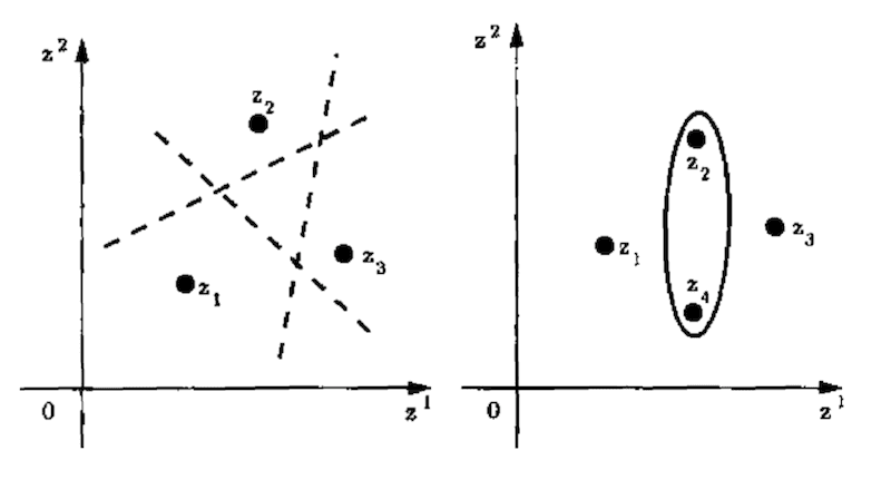
Example of a Line Hypothesis Shattering 3 Points and Ovals Shattering 4 Points
Taken from Page 81, The Nature of Statistical Learning Theory, 1999.
Therefore, the VC dimension of a machine learning algorithm is the largest number of data points in a dataset that a specific configuration of the algorithm (hyperparameters) or specific fit model can shatter.
A classifier that predicts the same value in all cases will have a VC dimension of 0, no points. A large VC dimension indicates that an algorithm is very flexible, although the flexibility may come at the cost of additional risk of overfitting.
The VC dimension is used as part of the PAC learning framework.
A key quantity in PAC learning is the Vapnik-Chervonenkis dimension, or VC dimension, which provides a measure of the complexity of a space of functions, and which allows the PAC framework to be extended to spaces containing an infinite number of functions.
— Page 344, Pattern Recognition and Machine Learning, 2006.
For more on PCA Learning, refer to the seminal book on the topic titled:
Further Reading
This section provides more resources on the topic if you are looking to go deeper.
Books
- Probably Approximately Correct: Nature’s Algorithms for Learning and Prospering in a Complex World, 2013.
- Artificial Intelligence: A Modern Approach, 3rd edition, 2009.
- An Introduction to Computational Learning Theory, 1994.
- Machine Learning: A Probabilistic Perspective, 2012.
- The Nature of Statistical Learning Theory, 1999.
- Pattern Recognition and Machine Learning, 2006.
- Machine Learning, 1997.
Articles
- Statistical learning theory, Wikipedia.
- Computational learning theory, Wikipedia.
- Probably approximately correct learning, Wikipedia.
- Vapnik–Chervonenkis theory, Wikipedia.
- Vapnik–Chervonenkis dimension, Wikipedia.
Summary
In this post, you discovered a gentle introduction to computational learning theory for machine learning.
Specifically, you learned:
- Computational learning theory uses formal methods to study learning tasks and learning algorithms.
- PAC learning provides a way to quantify the computational difficulty of a machine learning task.
- VC Dimension provides a way to quantify the computational capacity of a machine learning algorithm.
Do you have any questions?
Ask your questions in the comments below and I will do my best to answer.
The post A Gentle Introduction to Computational Learning Theory appeared first on Machine Learning Mastery.