
Author: Jason Brownlee
Random subspace ensembles consist of the same model fit on different randomly selected groups of input features (columns) in the training dataset.
There are many ways to choose groups of features in the training dataset, and feature selection is a popular class of data preparation techniques designed specifically for this purpose. The features selected by different configurations of the same feature selection method and different feature selection methods entirely can be used as the basis for ensemble learning.
In this tutorial, you will discover how to develop feature selection subspace ensembles with Python.
After completing this tutorial, you will know:
- Feature selection provides an alternative to random subspaces for selecting groups of input features.
- How to develop and evaluate ensembles composed of features selected by single feature selection techniques.
- How to develop and evaluate ensembles composed of features selected by multiple different feature selection techniques.
Let’s get started.

How to Develop a Feature Selection Subspace Ensemble in Python
Photo by Bernard Spragg. NZ, some rights reserved.
Tutorial Overview
This tutorial is divided into three parts; they are:
- Feature Selection Subspace Ensemble
- Single Feature Selection Method Ensembles
- ANOVA F-statistic Ensemble
- Mutual Information Ensemble
- Recursive Feature Selection Ensemble
- Combined Feature Selection Ensembles
- Ensemble With Fixed Number of Features
- Ensemble With Contiguous Number of Features
Feature Selection Subspace Ensemble
The random subspace method or random subspace ensemble is an approach to ensemble learning that fits a model on different groups of randomly selected columns in the training dataset.
The difference in the choice of columns used to train each model in the ensemble results in a diversity of models and their predictions. Each model performs well, although each performs differently, making different errors.
The training data is usually described by a set of features. Different subsets of features, or called subspaces, provide different views on the data. Therefore, individual learners trained from different subspaces are usually diverse.
— Page 116, Ensemble Methods, 2012.
The random subspace method is often used with decision trees and the predictions made by each tree are then combined using simple statistics, such as calculating the mode class label for classification or the mean prediction for regression.
Feature selection is a data preparation technique that attempts to select a subset of columns in a dataset that is most relevant to the target variable. Popular approaches involve using statistical measures, such as mutual information, and evaluating models on subsets of features and selecting the subset that results in the best performing model, called recursive feature elimination, or RFE for short.
Each feature selection method will have a different idea or informed guess about what features are most relevant to the target variable. Further, feature selection methods can be tailored to select a specific number of features from 1 to the total number of columns in the dataset, a hyperparameter that can be tuned as part of model selection.
Each set of selected features may be considered as a subset of the input feature space, much like a random subspace ensemble, although chosen using a metric instead of randomly. We can use features chosen by feature selection methods as a type of ensemble model.
There may be many ways that this could be implemented, but perhaps two natural approaches include:
- One Method: Generate a feature subspace for each number of features from 1 to the number of columns in the dataset, fit a model on each, and combine their predictions.
- Multiple Methods: Generate a feature subspace using multiple different feature selection methods, fit a model on each, and combine their predictions.
For lack of a better name, we can refer to this as a “Feature Selection Subspace Ensemble.”
We will explore this idea in this tutorial.
Let’s define a test problem as the basis for this exploration and establish a baseline in performance to see if it offers a benefit over a single model.
First, we can use the make_classification() function to create a synthetic binary classification problem with 1,000 examples and 20 input features, five of which are redundant.
The complete example is listed below.
# synthetic classification dataset
from sklearn.datasets import make_classification
# define dataset
X, y = make_classification(n_samples=1000, n_features=20, n_informative=15, n_redundant=5, random_state=5)
# summarize the dataset
print(X.shape, y.shape)
Running the example creates the dataset and summarizes the shape of the input and output components.
(1000, 20) (1000,)
Next, we can establish a baseline in performance. We will develop a decision tree for the dataset and evaluate it using repeated stratified k-fold cross-validation with three repeats and 10 folds.
The results will be reported as the mean and standard deviation of the classification accuracy across all repeats and folds.
The complete example is listed below.
# evaluate a decision tree on the classification dataset
from numpy import mean
from numpy import std
from sklearn.datasets import make_classification
from sklearn.model_selection import cross_val_score
from sklearn.model_selection import RepeatedStratifiedKFold
from sklearn.tree import DecisionTreeClassifier
# define dataset
X, y = make_classification(n_samples=1000, n_features=20, n_informative=15, n_redundant=5, random_state=5)
# define the random subspace ensemble model
model = DecisionTreeClassifier()
# define the evaluation method
cv = RepeatedStratifiedKFold(n_splits=10, n_repeats=3, random_state=1)
# evaluate the model on the dataset
n_scores = cross_val_score(model, X, y, scoring='accuracy', cv=cv, n_jobs=-1)
# report performance
print('Mean Accuracy: %.3f (%.3f)' % (mean(n_scores), std(n_scores)))
Running the example reports the mean and standard deviation classification accuracy.
Note: Your results may vary given the stochastic nature of the algorithm or evaluation procedure, or differences in numerical precision. Consider running the example a few times and compare the average outcome.
In this case, we can see that a single decision tree model achieves a classification accuracy of approximately 79.4 percent. We can use this as a baseline in performance to see if our feature selection ensembles are able to achieve better performance.
Mean Accuracy: 0.794 (0.046)
Next, let’s explore using different feature selection methods as the basis for ensembles.
Single Feature Selection Method Ensembles
In this section, we will explore creating an ensemble from the features selected by individual feature selection methods.
For a given feature selection method, we will apply it repeatedly with different numbers of selected features to create multiple feature subspaces. We will then train a model on each, in this case, a decision tree, and combine the predictions.
There are many ways to combine the predictions, but to keep things simple, we will use a voting ensemble that can be configured to use hard or soft voting for classification, or averaging for regression. To keep the examples simple, we will focus on classification and use hard voting, as the decision trees do not predict calibrated probabilities, making soft voting less appropriate.
To learn more about voting ensembles, see the tutorial:
Each model in the voting ensemble will be a Pipeline where the first step is a feature selection method, configured to select a specific number of features, followed by a decision tree classifier model.
We will create one feature selection subspace for each number of columns in the input dataset from 1 to the number of columns. This was chosen arbitrarily for simplicity and you might want to experiment with different numbers of features in the ensemble, such as odd numbers of features, or more elaborate methods.
As such, we can define a helper function named get_ensemble() that creates a voting ensemble with feature selection-based members for a given number of input features. We can then use this function as a template to explore using different feature selection methods.
# get a voting ensemble of models
def get_ensemble(n_features):
	# define the base models
	models = list()
	# enumerate the features in the training dataset
	for i in range(1, n_features+1):
		# create the feature selection transform
		fs = ...
		# create the model
		model = DecisionTreeClassifier()
		# create the pipeline
		pipe = Pipeline([('fs',fs), ('m', model)])
		# add as a tuple to the list of models for voting
		models.append((str(i),pipe))
	# define the voting ensemble
	ensemble = VotingClassifier(estimators=models, voting='hard')
	return ensemble
Given that we are working with a classification dataset, we will explore three different feature selection methods:
- ANOVA F-statistic.
- Mutual Information.
- Recursive Feature Selection.
Let’s take a closer look at each.
ANOVA F-statistic Ensemble
ANOVA is an acronym for “analysis of variance” and is a parametric statistical hypothesis test for determining whether the means from two or more samples of data (often three or more) come from the same distribution or not.
An F-statistic, or F-test, is a class of statistical tests that calculate the ratio between variances values, such as the variance from two different samples or the explained and unexplained variance by a statistical test, like ANOVA. The ANOVA method is a type of F-statistic referred to here as an ANOVA F-test.
The scikit-learn machine library provides an implementation of the ANOVA F-test in the f_classif() function. This function can be used in a feature selection strategy, such as selecting the top k most relevant features (largest values) via the SelectKBest class.
# get a voting ensemble of models
def get_ensemble(n_features):
	# define the base models
	models = list()
	# enumerate the features in the training dataset
	for i in range(1, n_features+1):
		# create the feature selection transform
		fs = SelectKBest(score_func=f_classif, k=i)
		# create the model
		model = DecisionTreeClassifier()
		# create the pipeline
		pipe = Pipeline([('fs',fs), ('m', model)])
		# add as a tuple to the list of models for voting
		models.append((str(i),pipe))
	# define the voting ensemble
	ensemble = VotingClassifier(estimators=models, voting='hard')
	return ensemble
Tying this together, the example below evaluates a voting ensemble composed of models fit on feature subspaces selected by the ANOVA F-statistic.
# example of an ensemble created from features selected with the anova f-statistic
from numpy import mean
from numpy import std
from sklearn.datasets import make_classification
from sklearn.model_selection import cross_val_score
from sklearn.model_selection import RepeatedStratifiedKFold
from sklearn.feature_selection import SelectKBest
from sklearn.feature_selection import f_classif
from sklearn.tree import DecisionTreeClassifier
from sklearn.ensemble import VotingClassifier
from sklearn.pipeline import Pipeline
from matplotlib import pyplot

# get a voting ensemble of models
def get_ensemble(n_features):
	# define the base models
	models = list()
	# enumerate the features in the training dataset
	for i in range(1, n_features+1):
		# create the feature selection transform
		fs = SelectKBest(score_func=f_classif, k=i)
		# create the model
		model = DecisionTreeClassifier()
		# create the pipeline
		pipe = Pipeline([('fs',fs), ('m', model)])
		# add as a tuple to the list of models for voting
		models.append((str(i),pipe))
	# define the voting ensemble
	ensemble = VotingClassifier(estimators=models, voting='hard')
	return ensemble

# define dataset
X, y = make_classification(n_samples=1000, n_features=20, n_informative=15, n_redundant=5, random_state=5)
# get the ensemble model
ensemble = get_ensemble(X.shape[1])
# define the evaluation method
cv = RepeatedStratifiedKFold(n_splits=10, n_repeats=3, random_state=1)
# evaluate the model on the dataset
n_scores = cross_val_score(ensemble, X, y, scoring='accuracy', cv=cv, n_jobs=-1)
# report performance
print('Mean Accuracy: %.3f (%.3f)' % (mean(n_scores), std(n_scores)))
Running the example reports the mean and standard deviation classification accuracy.
Note: Your results may vary given the stochastic nature of the algorithm or evaluation procedure, or differences in numerical precision. Consider running the example a few times and compare the average outcome.
In this case, we can see a lift in performance over a single model that achieved an accuracy of about 79.4 percent to about 83.2 percent using an ensemble of models on features selected by the ANOVA F-statistic.
Mean Accuracy: 0.832 (0.043)
Next, let’s explore using mutual information.
Mutual Information Ensemble
Mutual information from the field of information theory is the application of information gain (typically used in the construction of decision trees) to feature selection.
Mutual information is calculated between two variables and measures the reduction in uncertainty for one variable given a known value of the other variable. It is straightforward when considering the distribution of two discrete (categorical or ordinal) variables, such as categorical input and categorical output data. Nevertheless, it can be adapted for use with numerical input and categorical output.
The scikit-learn machine learning library provides an implementation of mutual information for feature selection with numeric input and categorical output variables via the mutual_info_classif() function. Like f_classif(), it can be used in the SelectKBest feature selection strategy (and other strategies).
# get a voting ensemble of models
def get_ensemble(n_features):
	# define the base models
	models = list()
	# enumerate the features in the training dataset
	for i in range(1, n_features+1):
		# create the feature selection transform
		fs = SelectKBest(score_func=mutual_info_classif, k=i)
		# create the model
		model = DecisionTreeClassifier()
		# create the pipeline
		pipe = Pipeline([('fs',fs), ('m', model)])
		# add as a tuple to the list of models for voting
		models.append((str(i),pipe))
	# define the voting ensemble
	ensemble = VotingClassifier(estimators=models, voting='hard')
	return ensemble
Tying this together, the example below evaluates a voting ensemble composed of models fit on feature subspaces selected by mutual information.
# example of an ensemble created from features selected with mutual information
from numpy import mean
from numpy import std
from sklearn.datasets import make_classification
from sklearn.model_selection import cross_val_score
from sklearn.model_selection import RepeatedStratifiedKFold
from sklearn.feature_selection import SelectKBest
from sklearn.feature_selection import mutual_info_classif
from sklearn.tree import DecisionTreeClassifier
from sklearn.ensemble import VotingClassifier
from sklearn.pipeline import Pipeline
from matplotlib import pyplot

# get a voting ensemble of models
def get_ensemble(n_features):
	# define the base models
	models = list()
	# enumerate the features in the training dataset
	for i in range(1, n_features+1):
		# create the feature selection transform
		fs = SelectKBest(score_func=mutual_info_classif, k=i)
		# create the model
		model = DecisionTreeClassifier()
		# create the pipeline
		pipe = Pipeline([('fs',fs), ('m', model)])
		# add as a tuple to the list of models for voting
		models.append((str(i),pipe))
	# define the voting ensemble
	ensemble = VotingClassifier(estimators=models, voting='hard')
	return ensemble

# define dataset
X, y = make_classification(n_samples=1000, n_features=20, n_informative=15, n_redundant=5, random_state=5)
# get the ensemble model
ensemble = get_ensemble(X.shape[1])
# define the evaluation method
cv = RepeatedStratifiedKFold(n_splits=10, n_repeats=3, random_state=1)
# evaluate the model on the dataset
n_scores = cross_val_score(ensemble, X, y, scoring='accuracy', cv=cv, n_jobs=-1)
# report performance
print('Mean Accuracy: %.3f (%.3f)' % (mean(n_scores), std(n_scores)))
Running the example reports the mean and standard deviation classification accuracy.
Note: Your results may vary given the stochastic nature of the algorithm or evaluation procedure, or differences in numerical precision. Consider running the example a few times and compare the average outcome.
In this case, we can see a lift in performance over using a single model, although slightly less than feature subspace selected, with the ANOVA F-statistic achieving a mean accuracy of about 82.7 percent.
Mean Accuracy: 0.827 (0.048)
Next, let’s explore subspaces selected using RFE.
Recursive Feature Selection Ensemble
Recursive Feature Elimination, or RFE for short, works by searching for a subset of features by starting with all features in the training dataset and successfully removing features until the desired number remains.
This is achieved by fitting the given machine learning algorithm used in the core of the model, ranking features by importance, discarding the least important features, and re-fitting the model. This process is repeated until a specified number of features remains.
For more on RFE, see the tutorial:
The RFE method is available via the RFE class in scikit-learn and can be used for feature selection directly. No need to combine it with the SelectKBest class.
# get a voting ensemble of models
def get_ensemble(n_features):
	# define the base models
	models = list()
	# enumerate the features in the training dataset
	for i in range(1, n_features+1):
		# create the feature selection transform
		fs = RFE(estimator=DecisionTreeClassifier(), n_features_to_select=i)
		# create the model
		model = DecisionTreeClassifier()
		# create the pipeline
		pipe = Pipeline([('fs',fs), ('m', model)])
		# add as a tuple to the list of models for voting
		models.append((str(i),pipe))
	# define the voting ensemble
	ensemble = VotingClassifier(estimators=models, voting='hard')
	return ensemble
Tying this together, the example below evaluates a voting ensemble composed of models fit on feature subspaces selected by RFE.
# example of an ensemble created from features selected with RFE
from numpy import mean
from numpy import std
from sklearn.datasets import make_classification
from sklearn.model_selection import cross_val_score
from sklearn.model_selection import RepeatedStratifiedKFold
from sklearn.feature_selection import RFE
from sklearn.tree import DecisionTreeClassifier
from sklearn.ensemble import VotingClassifier
from sklearn.pipeline import Pipeline
from matplotlib import pyplot

# get a voting ensemble of models
def get_ensemble(n_features):
	# define the base models
	models = list()
	# enumerate the features in the training dataset
	for i in range(1, n_features+1):
		# create the feature selection transform
		fs = RFE(estimator=DecisionTreeClassifier(), n_features_to_select=i)
		# create the model
		model = DecisionTreeClassifier()
		# create the pipeline
		pipe = Pipeline([('fs',fs), ('m', model)])
		# add as a tuple to the list of models for voting
		models.append((str(i),pipe))
	# define the voting ensemble
	ensemble = VotingClassifier(estimators=models, voting='hard')
	return ensemble

# define dataset
X, y = make_classification(n_samples=1000, n_features=20, n_informative=15, n_redundant=5, random_state=5)
# get the ensemble model
ensemble = get_ensemble(X.shape[1])
# define the evaluation method
cv = RepeatedStratifiedKFold(n_splits=10, n_repeats=3, random_state=1)
# evaluate the model on the dataset
n_scores = cross_val_score(ensemble, X, y, scoring='accuracy', cv=cv, n_jobs=-1)
# report performance
print('Mean Accuracy: %.3f (%.3f)' % (mean(n_scores), std(n_scores)))
Running the example reports the mean and standard deviation classification accuracy.
Note: Your results may vary given the stochastic nature of the algorithm or evaluation procedure, or differences in numerical precision. Consider running the example a few times and compare the average outcome.
In this case, we can see that the mean accuracy is similar to that seen with mutual information feature selection, with a score of about 82.3 percent.
Mean Accuracy: 0.823 (0.045)
This is a good start, and it might be interesting to see if better results can be achieved using ensembles composed of fewer members, e.g. every second, third, or fifth number of selected features.
Next, let’s see if we can improve results by combining models fit on feature subspaces selected by different feature selection methods.
Combined Feature Selection Ensembles
In the previous section, we saw that we can get a lift in performance over a single model by using a single feature selection method as the basis of an ensemble prediction for a dataset.
We would expect the predictions between many of the members of the ensemble to be correlated. This could be addressed by using different numbers of selected input features as the basis for the ensemble rather than a contiguous number of features from 1 to the number of columns.
An alternative approach to introducing diversity is to select feature subspaces using different feature selection methods.
We will explore two versions of this approach. With the first, we will select the same number of features from each method, and with the second, we will select a contiguous number of features from 1 to the number of columns for multiple methods.
Ensemble With Fixed Number of Features
In this section, we will make our first attempt at devising an ensemble using features selected by multiple feature selection techniques.
We will select an arbitrary number of features from the dataset, then use each of the three feature selection methods to select a feature subspace, fit a model of each, and use them as the basis for a voting ensemble.
The get_ensemble() function below implements this, taking the specified number of features to select with each method as an argument. The hope is that the features selected by each method are sufficiently different and sufficiently skillful to result in an effective ensemble.
# get a voting ensemble of models
def get_ensemble(n_features):
	# define the base models
	models = list()
	# anova
	fs = SelectKBest(score_func=f_classif, k=n_features)
	anova = Pipeline([('fs', fs), ('m', DecisionTreeClassifier())])
	models.append(('anova', anova))
	# mutual information
	fs = SelectKBest(score_func=mutual_info_classif, k=n_features)
	mutinfo = Pipeline([('fs', fs), ('m', DecisionTreeClassifier())])
	models.append(('mutinfo', mutinfo))
	# rfe
	fs = RFE(estimator=DecisionTreeClassifier(), n_features_to_select=n_features)
	rfe = Pipeline([('fs', fs), ('m', DecisionTreeClassifier())])
	models.append(('rfe', rfe))
	# define the voting ensemble
	ensemble = VotingClassifier(estimators=models, voting='hard')
	return ensemble
Tying this together, the example below evaluates an ensemble of a fixed number of features selected using different feature selection methods.
# ensemble of a fixed number features selected by different feature selection methods
from numpy import mean
from numpy import std
from sklearn.datasets import make_classification
from sklearn.model_selection import cross_val_score
from sklearn.model_selection import RepeatedStratifiedKFold
from sklearn.feature_selection import RFE
from sklearn.feature_selection import SelectKBest
from sklearn.feature_selection import mutual_info_classif
from sklearn.feature_selection import f_classif
from sklearn.tree import DecisionTreeClassifier
from sklearn.ensemble import VotingClassifier
from sklearn.pipeline import Pipeline
from matplotlib import pyplot

# get a voting ensemble of models
def get_ensemble(n_features):
	# define the base models
	models = list()
	# anova
	fs = SelectKBest(score_func=f_classif, k=n_features)
	anova = Pipeline([('fs', fs), ('m', DecisionTreeClassifier())])
	models.append(('anova', anova))
	# mutual information
	fs = SelectKBest(score_func=mutual_info_classif, k=n_features)
	mutinfo = Pipeline([('fs', fs), ('m', DecisionTreeClassifier())])
	models.append(('mutinfo', mutinfo))
	# rfe
	fs = RFE(estimator=DecisionTreeClassifier(), n_features_to_select=n_features)
	rfe = Pipeline([('fs', fs), ('m', DecisionTreeClassifier())])
	models.append(('rfe', rfe))
	# define the voting ensemble
	ensemble = VotingClassifier(estimators=models, voting='hard')
	return ensemble

# define dataset
X, y = make_classification(n_samples=1000, n_features=20, n_informative=15, n_redundant=5, random_state=1)
# get the ensemble model
ensemble = get_ensemble(15)
# define the evaluation method
cv = RepeatedStratifiedKFold(n_splits=10, n_repeats=3, random_state=1)
# evaluate the model on the dataset
n_scores = cross_val_score(ensemble, X, y, scoring='accuracy', cv=cv, n_jobs=-1)
# report performance
print('Mean Accuracy: %.3f (%.3f)' % (mean(n_scores), std(n_scores)))
Running the example reports the mean and standard deviation classification accuracy.
Note: Your results may vary given the stochastic nature of the algorithm or evaluation procedure, or differences in numerical precision. Consider running the example a few times and compare the average outcome.
In this case, we can see a modest lift in performance over the techniques considered in the previous section, resulting in a mean classification accuracy of about 83.9 percent.
Mean Accuracy: 0.839 (0.044)
A more fair comparison might be to compare this result to each individual model that comprises the ensemble.
The updated example performs exactly this comparison.
# comparison of ensemble of a fixed number features to single models fit on each set of features
from numpy import mean
from numpy import std
from sklearn.datasets import make_classification
from sklearn.model_selection import cross_val_score
from sklearn.model_selection import RepeatedStratifiedKFold
from sklearn.feature_selection import RFE
from sklearn.feature_selection import SelectKBest
from sklearn.feature_selection import mutual_info_classif
from sklearn.feature_selection import f_classif
from sklearn.tree import DecisionTreeClassifier
from sklearn.ensemble import VotingClassifier
from sklearn.pipeline import Pipeline
from matplotlib import pyplot

# get a voting ensemble of models
def get_ensemble(n_features):
	# define the base models
	models, names = list(), list()
	# anova
	fs = SelectKBest(score_func=f_classif, k=n_features)
	anova = Pipeline([('fs', fs), ('m', DecisionTreeClassifier())])
	models.append(('anova', anova))
	names.append('anova')
	# mutual information
	fs = SelectKBest(score_func=mutual_info_classif, k=n_features)
	mutinfo = Pipeline([('fs', fs), ('m', DecisionTreeClassifier())])
	models.append(('mutinfo', mutinfo))
	names.append('mutinfo')
	# rfe
	fs = RFE(estimator=DecisionTreeClassifier(), n_features_to_select=n_features)
	rfe = Pipeline([('fs', fs), ('m', DecisionTreeClassifier())])
	models.append(('rfe', rfe))
	names.append('rfe')
	# define the voting ensemble
	ensemble = VotingClassifier(estimators=models, voting='hard')
	names.append('ensemble')
	return names, [anova, mutinfo, rfe, ensemble]

# define dataset
X, y = make_classification(n_samples=1000, n_features=20, n_informative=15, n_redundant=5, random_state=1)
# get the ensemble model
names, models = get_ensemble(15)
# evaluate each model
results = list()
for model,name in zip(models,names):
	# define the evaluation method
	cv = RepeatedStratifiedKFold(n_splits=10, n_repeats=3, random_state=1)
	# evaluate the model on the dataset
	n_scores = cross_val_score(model, X, y, scoring='accuracy', cv=cv, n_jobs=-1)
	# report performance
	print('>%s: %.3f (%.3f)' % (name, mean(n_scores), std(n_scores)))
	results.append(n_scores)
# plot the results for comparison
pyplot.boxplot(results, labels=names)
pyplot.show()
Running the example reports the mean performance of each single model fit on the selected features and ends with the performance of the ensemble that combines all three models.
Note: Your results may vary given the stochastic nature of the algorithm or evaluation procedure, or differences in numerical precision. Consider running the example a few times and compare the average outcome.
In this case, the results suggest that the ensemble of the models fit on the selected features performs better than any single model in the ensemble, as we might hope.
>anova: 0.811 (0.048)
>mutinfo: 0.807 (0.041)
>rfe: 0.825 (0.043)
>ensemble: 0.837 (0.040)
A figure is created to show box and whisker plots for each set of results, allowing the distribution accuracy scores to be compared directly.
We can see that the distribution for the ensemble both skews higher and has a larger median classification accuracy (orange line), visually confirming the finding.
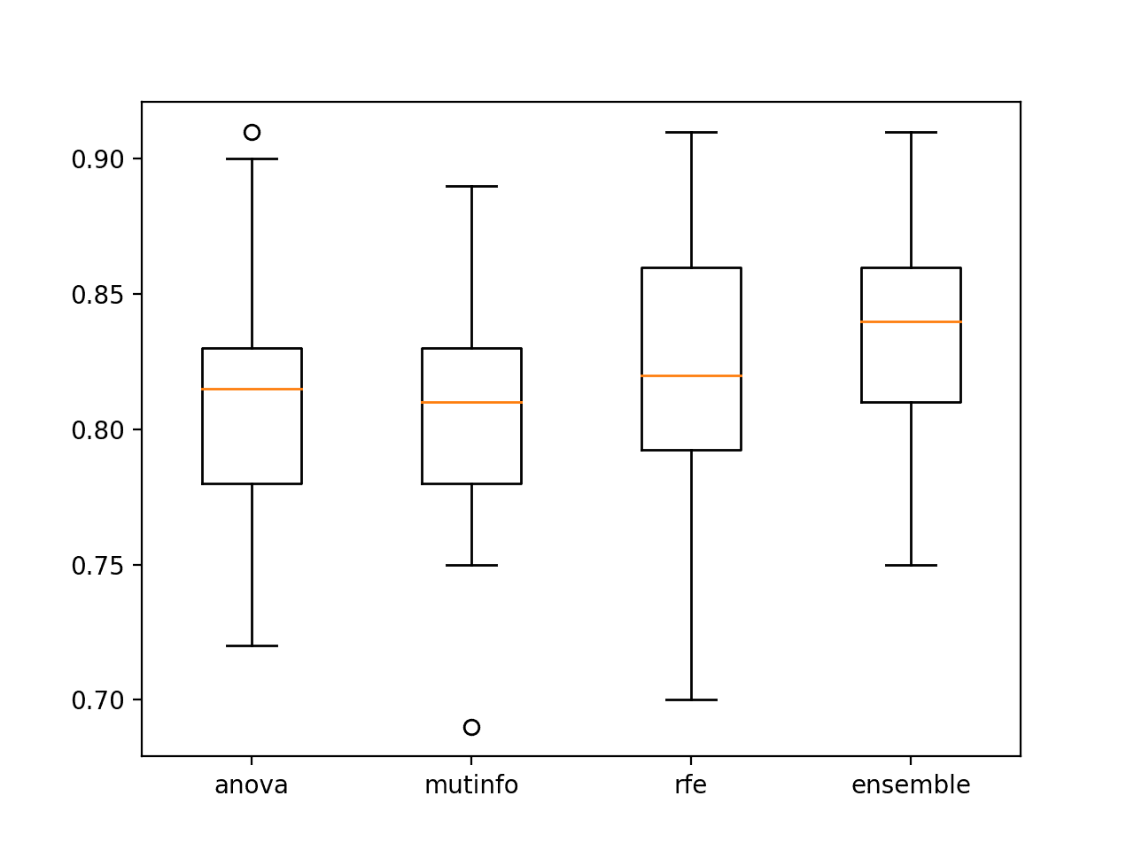
Box and Whisker Plots of Accuracy of Singles Model Fit On Selected Features vs. Ensemble
Next, let’s explore adding multiple members for each feature selection method.
Ensemble With Contiguous Number of Features
We can combine the experiments from the previous section with the above experiment.
Specifically, we can select multiple feature subspaces using each feature selection method, fit a model on each, and add all of the models to a single ensemble.
In this case, we will select subspace as we did in the previous section from 1 to the number of columns in the dataset, although in this case, repeat the process with each feature selection method.
# get a voting ensemble of models
def get_ensemble(n_features_start, n_features_end):
	# define the base models
	models = list()
	for i in range(n_features_start, n_features_end+1):
		# anova
		fs = SelectKBest(score_func=f_classif, k=i)
		anova = Pipeline([('fs', fs), ('m', DecisionTreeClassifier())])
		models.append(('anova'+str(i), anova))
		# mutual information
		fs = SelectKBest(score_func=mutual_info_classif, k=i)
		mutinfo = Pipeline([('fs', fs), ('m', DecisionTreeClassifier())])
		models.append(('mutinfo'+str(i), mutinfo))
		# rfe
		fs = RFE(estimator=DecisionTreeClassifier(), n_features_to_select=i)
		rfe = Pipeline([('fs', fs), ('m', DecisionTreeClassifier())])
		models.append(('rfe'+str(i), rfe))
	# define the voting ensemble
	ensemble = VotingClassifier(estimators=models, voting='hard')
	return ensemble
The hope is that the diversity of the selected features across the feature selection methods results in a further lift in ensemble performance.
Tying this together, the complete example is listed below.
# ensemble of many subsets of features selected by multiple feature selection methods
from numpy import mean
from numpy import std
from sklearn.datasets import make_classification
from sklearn.model_selection import cross_val_score
from sklearn.model_selection import RepeatedStratifiedKFold
from sklearn.feature_selection import RFE
from sklearn.feature_selection import SelectKBest
from sklearn.feature_selection import mutual_info_classif
from sklearn.feature_selection import f_classif
from sklearn.tree import DecisionTreeClassifier
from sklearn.ensemble import VotingClassifier
from sklearn.pipeline import Pipeline
from matplotlib import pyplot

# get a voting ensemble of models
def get_ensemble(n_features_start, n_features_end):
	# define the base models
	models = list()
	for i in range(n_features_start, n_features_end+1):
		# anova
		fs = SelectKBest(score_func=f_classif, k=i)
		anova = Pipeline([('fs', fs), ('m', DecisionTreeClassifier())])
		models.append(('anova'+str(i), anova))
		# mutual information
		fs = SelectKBest(score_func=mutual_info_classif, k=i)
		mutinfo = Pipeline([('fs', fs), ('m', DecisionTreeClassifier())])
		models.append(('mutinfo'+str(i), mutinfo))
		# rfe
		fs = RFE(estimator=DecisionTreeClassifier(), n_features_to_select=i)
		rfe = Pipeline([('fs', fs), ('m', DecisionTreeClassifier())])
		models.append(('rfe'+str(i), rfe))
	# define the voting ensemble
	ensemble = VotingClassifier(estimators=models, voting='hard')
	return ensemble

# define dataset
X, y = make_classification(n_samples=1000, n_features=20, n_informative=15, n_redundant=5, random_state=1)
# get the ensemble model
ensemble = get_ensemble(1, 20)
# define the evaluation method
cv = RepeatedStratifiedKFold(n_splits=10, n_repeats=3, random_state=1)
# evaluate the model on the dataset
n_scores = cross_val_score(ensemble, X, y, scoring='accuracy', cv=cv, n_jobs=-1)
# report performance
print('Mean Accuracy: %.3f (%.3f)' % (mean(n_scores), std(n_scores)))
Running the example reports the mean and standard deviation classification accuracy of the ensemble.
Note: Your results may vary given the stochastic nature of the algorithm or evaluation procedure, or differences in numerical precision. Consider running the example a few times and compare the average outcome.
In this case, we can see a further lift of performance as we hoped, where the combined ensemble resulted in a mean classification accuracy of about 86.0 percent.
Mean Accuracy: 0.860 (0.036)
The use of feature selection for selecting subspaces of input features may provide an interesting alternative or perhaps complement to selecting random subspaces.
Further Reading
This section provides more resources on the topic if you are looking to go deeper.
Tutorials
- How to Develop Voting Ensembles With Python
- Recursive Feature Elimination (RFE) for Feature Selection in Python
- How to Perform Feature Selection With Numerical Input Data
Books
- Pattern Classification Using Ensemble Methods, 2010.
- Ensemble Methods, 2012.
- Ensemble Machine Learning, 2012.
APIs
- sklearn.feature_selection.f_classif API.
- sklearn.feature_selection.mutual_info_classif API.
- sklearn.feature_selection.SelectKBest API.
- sklearn.feature_selection.RFE API.
Articles
Summary
In this tutorial, you discovered how to develop feature selection subspace ensembles with Python.
Specifically, you learned:
- Feature selection provides an alternative to random subspaces for selecting groups of input features.
- How to develop and evaluate ensembles composed of features selected by single feature selection techniques.
- How to develop and evaluate ensembles composed of features selected by multiple different feature selection techniques.
Do you have any questions?
Ask your questions in the comments below and I will do my best to answer.
The post How to Develop a Feature Selection Subspace Ensemble in Python appeared first on Machine Learning Mastery.