
Author: Jason Brownlee
How to Optimize a Function with One Variable?
Univariate function optimization involves finding the input to a function that results in the optimal output from an objective function.
This is a common procedure in machine learning when fitting a model with one parameter or tuning a model that has a single hyperparameter.
An efficient algorithm is required to solve optimization problems of this type that will find the best solution with the minimum number of evaluations of the objective function, given that each evaluation of the objective function could be computationally expensive, such as fitting and evaluating a model on a dataset.
This excludes expensive grid search and random search algorithms and in favor of efficient algorithms like Brent’s method.
In this tutorial, you will discover how to perform univariate function optimization in Python.
After completing this tutorial, you will know:
- Univariate function optimization involves finding an optimal input for an objective function that takes a single continuous argument.
- How to perform univariate function optimization for an unconstrained convex function.
- How to perform univariate function optimization for an unconstrained non-convex function.
Let’s get started.

Univariate Function Optimization in Python
Photo by Robert Haandrikman, some rights reserved.
Tutorial Overview
This tutorial is divided into three parts; they are:
- Univariate Function Optimization
- Convex Univariate Function Optimization
- Non-Convex Univariate Function Optimization
Univariate Function Optimization
We may need to find an optimal value of a function that takes a single parameter.
In machine learning, this may occur in many situations, such as:
- Finding the coefficient of a model to fit to a training dataset.
- Finding the value of a single hyperparameter that results in the best model performance.
This is called univariate function optimization.
We may be interested in the minimum outcome or maximum outcome of the function, although this can be simplified to minimization as a maximizing function can be made minimizing by adding a negative sign to all outcomes of the function.
There may or may not be limits on the inputs to the function, so-called unconstrained or constrained optimization, and we assume that small changes in input correspond to small changes in the output of the function, e.g. that it is smooth.
The function may or may not have a single optima, although we prefer that it does have a single optima and that shape of the function looks like a large basin. If this is the case, we know we can sample the function at one point and find the path down to the minima of the function. Technically, this is referred to as a convex function for minimization (concave for maximization), and functions that don’t have this basin shape are referred to as non-convex.
- Convex Target Function: There is a single optima and the shape of the target function leads to this optima.
Nevertheless, the target function is sufficiently complex that we don’t know the derivative, meaning we cannot just use calculus to analytically compute the minimum or maximum of the function where the gradient is zero. This is referred to as a function that is non-differentiable.
Although we might be able to sample the function with candidate values, we don’t know the input that will result in the best outcome. This may be because of the many reasons it is expensive to evaluate candidate solutions.
Therefore, we require an algorithm that efficiently samples input values to the function.
One approach to solving univariate function optimization problems is to use Brent’s method.
Brent’s method is an optimization algorithm that combines a bisecting algorithm (Dekker’s method) and inverse quadratic interpolation. It can be used for constrained and unconstrained univariate function optimization.
The Brent-Dekker method is an extension of the bisection method. It is a root-finding algorithm that combines elements of the secant method and inverse quadratic interpolation. It has reliable and fast convergence properties, and it is the univariate optimization algorithm of choice in many popular numerical optimization packages.
— Pages 49-51, Algorithms for Optimization, 2019.
Bisecting algorithms use a bracket (lower and upper) of input values and split up the input domain, bisecting it in order to locate where in the domain the optima is located, much like a binary search. Dekker’s method is one way this is achieved efficiently for a continuous domain.
Dekker’s method gets stuck on non-convex problems. Brent’s method modifies Dekker’s method to avoid getting stuck and also approximates the second derivative of the objective function (called the Secant Method) in an effort to accelerate the search.
As such, Brent’s method for univariate function optimization is generally preferred over most other univariate function optimization algorithms given its efficiency.
Brent’s method is available in Python via the minimize_scalar() SciPy function that takes the name of the function to be minimized. If your target function is constrained to a range, it can be specified via the “bounds” argument.
It returns an OptimizeResult object that is a dictionary containing the solution. Importantly, the ‘x‘ key summarizes the input for the optima, the ‘fun‘ key summarizes the function output for the optima, and the ‘nfev‘ summarizes the number of evaluations of the target function that were performed.
...
# minimize the function
result = minimize_scalar(objective, method='brent')
Now that we know how to perform univariate function optimization in Python, let’s look at some examples.
Convex Univariate Function Optimization
In this section, we will explore how to solve a convex univariate function optimization problem.
First, we can define a function that implements our function.
In this case, we will use a simple offset version of the x^2 function e.g. a simple parabola (u-shape) function. It is a minimization objective function with an optima at -5.0.
# objective function
def objective(x):
	return (5.0 + x)**2.0
We can plot a coarse grid of this function with input values from -10 to 10 to get an idea of the shape of the target function.
The complete example is listed below.
# plot a convex target function
from numpy import arange
from matplotlib import pyplot

# objective function
def objective(x):
	return (5.0 + x)**2.0

# define range
r_min, r_max = -10.0, 10.0
# prepare inputs
inputs = arange(r_min, r_max, 0.1)
# compute targets
targets = [objective(x) for x in inputs]
# plot inputs vs target
pyplot.plot(inputs, targets, '--')
pyplot.show()
Running the example evaluates input values in our specified range using our target function and creates a plot of the function inputs to function outputs.
We can see the U-shape of the function and that the objective is at -5.0.
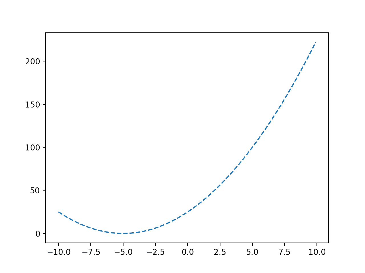
Line Plot of a Convex Objective Function
Note: in a real optimization problem, we would not be able to perform so many evaluations of the objective function so easily. This simple function is used for demonstration purposes so we can learn how to use the optimization algorithm.
Next, we can use the optimization algorithm to find the optima.
...
# minimize the function
result = minimize_scalar(objective, method='brent')
Once optimized, we can summarize the result, including the input and evaluation of the optima and the number of function evaluations required to locate the optima.
...
# summarize the result
opt_x, opt_y = result['x'], result['fun']
print('Optimal Input x: %.6f' % opt_x)
print('Optimal Output f(x): %.6f' % opt_y)
print('Total Evaluations n: %d' % result['nfev'])
Finally, we can plot the function again and mark the optima to confirm it was located in the place we expected for this function.
...
# define the range
r_min, r_max = -10.0, 10.0
# prepare inputs
inputs = arange(r_min, r_max, 0.1)
# compute targets
targets = [objective(x) for x in inputs]
# plot inputs vs target
pyplot.plot(inputs, targets, '--')
# plot the optima
pyplot.plot([opt_x], [opt_y], 's', color='r')
# show the plot
pyplot.show()
The complete example of optimizing an unconstrained convex univariate function is listed below.
# optimize convex objective function
from numpy import arange
from scipy.optimize import minimize_scalar
from matplotlib import pyplot

# objective function
def objective(x):
	return (5.0 + x)**2.0

# minimize the function
result = minimize_scalar(objective, method='brent')
# summarize the result
opt_x, opt_y = result['x'], result['fun']
print('Optimal Input x: %.6f' % opt_x)
print('Optimal Output f(x): %.6f' % opt_y)
print('Total Evaluations n: %d' % result['nfev'])
# define the range
r_min, r_max = -10.0, 10.0
# prepare inputs
inputs = arange(r_min, r_max, 0.1)
# compute targets
targets = [objective(x) for x in inputs]
# plot inputs vs target
pyplot.plot(inputs, targets, '--')
# plot the optima
pyplot.plot([opt_x], [opt_y], 's', color='r')
# show the plot
pyplot.show()
Running the example first solves the optimization problem and reports the result.
Note: Your results may vary given the stochastic nature of the algorithm or evaluation procedure, or differences in numerical precision. Consider running the example a few times and compare the average outcome.
In this case, we can see that the optima was located after 10 evaluations of the objective function with an input of -5.0, achieving an objective function value of 0.0.
Optimal Input x: -5.000000
Optimal Output f(x): 0.000000
Total Evaluations n: 10
A plot of the function is created again and this time, the optima is marked as a red square.

Line Plot of a Convex Objective Function with Optima Marked
Non-Convex Univariate Function Optimization
A convex function is one that does not resemble a basin, meaning that it may have more than one hill or valley.
This can make it more challenging to locate the global optima as the multiple hills and valleys can cause the search to get stuck and report a false or local optima instead.
We can define a non-convex univariate function as follows.
# objective function
def objective(x):
	return (x - 2.0) * x * (x + 2.0)**2.0
We can sample this function and create a line plot of input values to objective values.
The complete example is listed below.
# plot a non-convex univariate function
from numpy import arange
from matplotlib import pyplot

# objective function
def objective(x):
	return (x - 2.0) * x * (x + 2.0)**2.0

# define range
r_min, r_max = -3.0, 2.5
# prepare inputs
inputs = arange(r_min, r_max, 0.1)
# compute targets
targets = [objective(x) for x in inputs]
# plot inputs vs target
pyplot.plot(inputs, targets, '--')
pyplot.show()
Running the example evaluates input values in our specified range using our target function and creates a plot of the function inputs to function outputs.
We can see a function with one false optima around -2.0 and a global optima around 1.2.
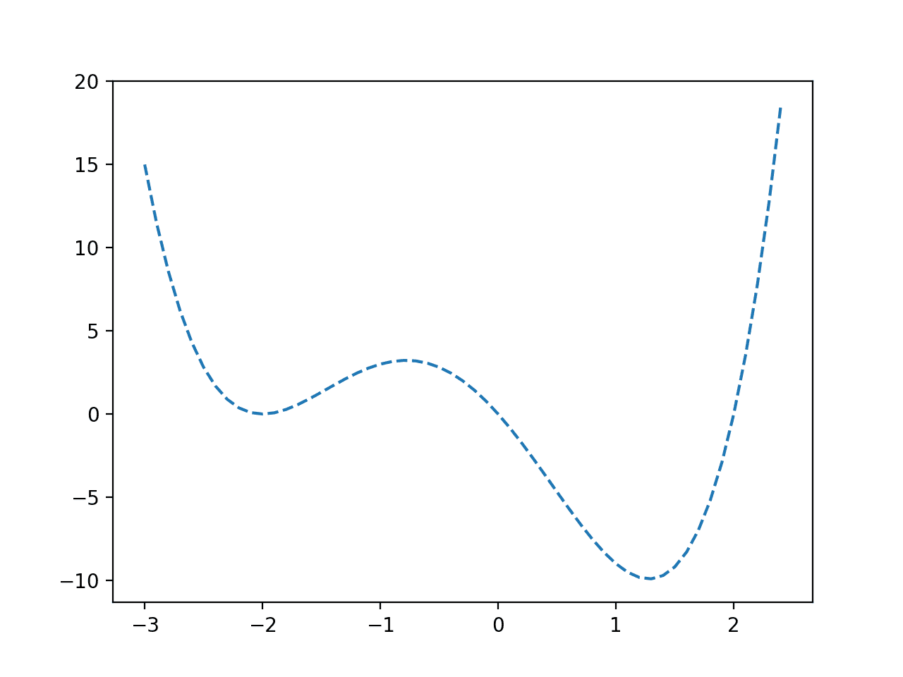
Line Plot of a Non-Convex Objective Function
Note: in a real optimization problem, we would not be able to perform so many evaluations of the objective function so easily. This simple function is used for demonstration purposes so we can learn how to use the optimization algorithm.
Next, we can use the optimization algorithm to find the optima.
As before, we can call the minimize_scalar() function to optimize the function, then summarize the result and plot the optima on a line plot.
The complete example of optimization of an unconstrained non-convex univariate function is listed below.
# optimize non-convex objective function
from numpy import arange
from scipy.optimize import minimize_scalar
from matplotlib import pyplot

# objective function
def objective(x):
	return (x - 2.0) * x * (x + 2.0)**2.0

# minimize the function
result = minimize_scalar(objective, method='brent')
# summarize the result
opt_x, opt_y = result['x'], result['fun']
print('Optimal Input x: %.6f' % opt_x)
print('Optimal Output f(x): %.6f' % opt_y)
print('Total Evaluations n: %d' % result['nfev'])
# define the range
r_min, r_max = -3.0, 2.5
# prepare inputs
inputs = arange(r_min, r_max, 0.1)
# compute targets
targets = [objective(x) for x in inputs]
# plot inputs vs target
pyplot.plot(inputs, targets, '--')
# plot the optima
pyplot.plot([opt_x], [opt_y], 's', color='r')
# show the plot
pyplot.show()
Running the example first solves the optimization problem and reports the result.
Want to Get Started With Ensemble Learning?
Take my free 7-day email crash course now (with sample code).
Click to sign-up and also get a free PDF Ebook version of the course.
In this case, we can see that the optima was located after 15 evaluations of the objective function with an input of about 1.28, achieving an objective function value of about -9.91.
Optimal Input x: 1.280776
Optimal Output f(x): -9.914950
Total Evaluations n: 15
A plot of the function is created again, and this time, the optima is marked as a red square.
We can see that the optimization was not deceived by the false optima and successfully located the global optima.
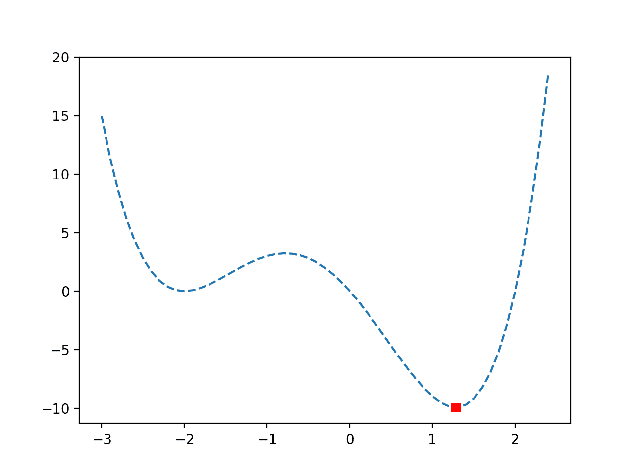
Line Plot of a Non-Convex Objective Function with Optima Marked
Further Reading
This section provides more resources on the topic if you are looking to go deeper.
Books
- Algorithms for Optimization, 2019.
APIs
- Optimization (scipy.optimize).
- Optimization and root finding (scipy.optimize)
- scipy.optimize.minimize_scalar API.
Articles
Summary
In this tutorial, you discovered how to perform univariate function optimization in Python.
Specifically, you learned:
- Univariate function optimization involves finding an optimal input for an objective function that takes a single continuous argument.
- How to perform univariate function optimization for an unconstrained convex function.
- How to perform univariate function optimization for an unconstrained non-convex function.
Do you have any questions?
Ask your questions in the comments below and I will do my best to answer.
The post Univariate Function Optimization in Python appeared first on Machine Learning Mastery.