
Author: Jason Brownlee
Evolution strategies is a stochastic global optimization algorithm.
It is an evolutionary algorithm related to others, such as the genetic algorithm, although it is designed specifically for continuous function optimization.
In this tutorial, you will discover how to implement the evolution strategies optimization algorithm.
After completing this tutorial, you will know:
- Evolution Strategies is a stochastic global optimization algorithm inspired by the biological theory of evolution by natural selection.
- There is a standard terminology for Evolution Strategies and two common versions of the algorithm referred to as (mu, lambda)-ES and (mu + lambda)-ES.
- How to implement and apply the Evolution Strategies algorithm to continuous objective functions.
Let’s get started.

Evolution Strategies From Scratch in Python
Photo by Alexis A. Bermúdez, some rights reserved.
Tutorial Overview
This tutorial is divided into three parts; they are:
- Evolution Strategies
- Develop a (mu, lambda)-ES
- Develop a (mu + lambda)-ES
Evolution Strategies
Evolution Strategies, sometimes referred to as Evolution Strategy (singular) or ES, is a stochastic global optimization algorithm.
The technique was developed in the 1960s to be implemented manually by engineers for minimal drag designs in a wind tunnel.
The family of algorithms known as Evolution Strategies (ES) were developed by Ingo Rechenberg and Hans-Paul Schwefel at the Technical University of Berlin in the mid 1960s.
— Page 31, Essentials of Metaheuristics, 2011.
Evolution Strategies is a type of evolutionary algorithm and is inspired by the biological theory of evolution by means of natural selection. Unlike other evolutionary algorithms, it does not use any form of crossover; instead, modification of candidate solutions is limited to mutation operators. In this way, Evolution Strategies may be thought of as a type of parallel stochastic hill climbing.
The algorithm involves a population of candidate solutions that initially are randomly generated. Each iteration of the algorithm involves first evaluating the population of solutions, then deleting all but a subset of the best solutions, referred to as truncation selection. The remaining solutions (the parents) each are used as the basis for generating a number of new candidate solutions (mutation) that replace or compete with the parents for a position in the population for consideration in the next iteration of the algorithm (generation).
There are a number of variations of this procedure and a standard terminology to summarize the algorithm. The size of the population is referred to as lambda and the number of parents selected each iteration is referred to as mu.
The number of children created from each parent is calculated as (lambda / mu) and parameters should be chosen so that the division has no remainder.
- mu: The number of parents selected each iteration.
- lambda: Size of the population.
- lambda / mu: Number of children generated from each selected parent.
A bracket notation is used to describe the algorithm configuration, e.g. (mu, lambda)-ES. For example, if mu=5 and lambda=20, then it would be summarized as (5, 20)-ES. A comma (,) separating the mu and lambda parameters indicates that the children replace the parents directly each iteration of the algorithm.
- (mu, lambda)-ES: A version of evolution strategies where children replace parents.
A plus (+) separation of the mu and lambda parameters indicates that the children and the parents together will define the population for the next iteration.
- (mu + lambda)-ES: A version of evolution strategies where children and parents are added to the population.
A stochastic hill climbing algorithm can be implemented as an Evolution Strategy and would have the notation (1 + 1)-ES.
This is the simile or canonical ES algorithm and there are many extensions and variants described in the literature.
Now that we are familiar with Evolution Strategies we can explore how to implement the algorithm.
Develop a (mu, lambda)-ES
In this section, we will develop a (mu, lambda)-ES, that is, a version of the algorithm where children replace parents.
First, let’s define a challenging optimization problem as the basis for implementing the algorithm.
The Ackley function is an example of a multimodal objective function that has a single global optima and multiple local optima in which a local search might get stuck.
As such, a global optimization technique is required. It is a two-dimensional objective function that has a global optima at [0,0], which evaluates to 0.0.
The example below implements the Ackley and creates a three-dimensional surface plot showing the global optima and multiple local optima.
# ackley multimodal function
from numpy import arange
from numpy import exp
from numpy import sqrt
from numpy import cos
from numpy import e
from numpy import pi
from numpy import meshgrid
from matplotlib import pyplot
from mpl_toolkits.mplot3d import Axes3D

# objective function
def objective(x, y):
	return -20.0 * exp(-0.2 * sqrt(0.5 * (x**2 + y**2))) - exp(0.5 * (cos(2 * pi * x) + cos(2 * pi * y))) + e + 20

# define range for input
r_min, r_max = -5.0, 5.0
# sample input range uniformly at 0.1 increments
xaxis = arange(r_min, r_max, 0.1)
yaxis = arange(r_min, r_max, 0.1)
# create a mesh from the axis
x, y = meshgrid(xaxis, yaxis)
# compute targets
results = objective(x, y)
# create a surface plot with the jet color scheme
figure = pyplot.figure()
axis = figure.gca(projection='3d')
axis.plot_surface(x, y, results, cmap='jet')
# show the plot
pyplot.show()
Running the example creates the surface plot of the Ackley function showing the vast number of local optima.
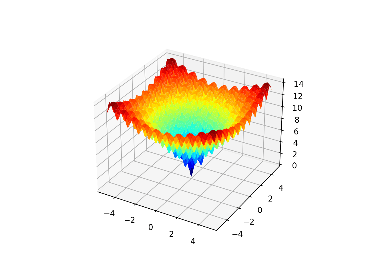
3D Surface Plot of the Ackley Multimodal Function
We will be generating random candidate solutions as well as modified versions of existing candidate solutions. It is important that all candidate solutions are within the bounds of the search problem.
To achieve this, we will develop a function to check whether a candidate solution is within the bounds of the search and then discard it and generate another solution if it is not.
The in_bounds() function below will take a candidate solution (point) and the definition of the bounds of the search space (bounds) and return True if the solution is within the bounds of the search or False otherwise.
# check if a point is within the bounds of the search
def in_bounds(point, bounds):
	# enumerate all dimensions of the point
	for d in range(len(bounds)):
		# check if out of bounds for this dimension
		if point[d] < bounds[d, 0] or point[d] > bounds[d, 1]:
			return False
	return True
We can then use this function when generating the initial population of “lam” (e.g. lambda) random candidate solutions.
For example:
...
# initial population
population = list()
for _ in range(lam):
	candidate = None
	while candidate is None or not in_bounds(candidate, bounds):
		candidate = bounds[:, 0] + rand(len(bounds)) * (bounds[:, 1] - bounds[:, 0])
	population.append(candidate)
Next, we can iterate over a fixed number of iterations of the algorithm. Each iteration first involves evaluating each candidate solution in the population.
We will calculate the scores and store them in a separate parallel list.
...
# evaluate fitness for the population
scores = [objective(c) for c in population]
Next, we need to select the “mu” parents with the best scores, lowest scores in this case, as we are minimizing the objective function.
We will do this in two steps. First, we will rank the candidate solutions based on their scores in ascending order so that the solution with the lowest score has a rank of 0, the next has a rank 1, and so on. We can use a double call of the argsort function to achieve this.
We will then use the ranks and select those parents that have a rank below the value “mu.” This means if mu is set to 5 to select 5 parents, only those parents with a rank between 0 and 4 will be selected.
...
# rank scores in ascending order
ranks = argsort(argsort(scores))
# select the indexes for the top mu ranked solutions
selected = [i for i,_ in enumerate(ranks) if ranks[i] < mu]
We can then create children for each selected parent.
First, we must calculate the total number of children to create per parent.
...
# calculate the number of children per parent
n_children = int(lam / mu)
We can then iterate over each parent and create modified versions of each.
We will create children using a similar technique used in stochastic hill climbing. Specifically, each variable will be sampled using a Gaussian distribution with the current value as the mean and the standard deviation provided as a “step size” hyperparameter.
...
# create children for parent
for _ in range(n_children):
	child = None
	while child is None or not in_bounds(child, bounds):
		child = population[i] + randn(len(bounds)) * step_size
We can also check if each selected parent is better than the best solution seen so far so that we can return the best solution at the end of the search.
...
# check if this parent is the best solution ever seen
if scores[i] < best_eval:
	best, best_eval = population[i], scores[i]
	print('%d, Best: f(%s) = %.5f' % (epoch, best, best_eval))
The created children can be added to a list and we can replace the population with the list of children at the end of the algorithm iteration.
...
# replace population with children
population = children
We can tie all of this together into a function named es_comma() that performs the comma version of the Evolution Strategy algorithm.
The function takes the name of the objective function, the bounds of the search space, the number of iterations, the step size, and the mu and lambda hyperparameters and returns the best solution found during the search and its evaluation.
# evolution strategy (mu, lambda) algorithm
def es_comma(objective, bounds, n_iter, step_size, mu, lam):
	best, best_eval = None, 1e+10
	# calculate the number of children per parent
	n_children = int(lam / mu)
	# initial population
	population = list()
	for _ in range(lam):
		candidate = None
		while candidate is None or not in_bounds(candidate, bounds):
			candidate = bounds[:, 0] + rand(len(bounds)) * (bounds[:, 1] - bounds[:, 0])
		population.append(candidate)
	# perform the search
	for epoch in range(n_iter):
		# evaluate fitness for the population
		scores = [objective(c) for c in population]
		# rank scores in ascending order
		ranks = argsort(argsort(scores))
		# select the indexes for the top mu ranked solutions
		selected = [i for i,_ in enumerate(ranks) if ranks[i] < mu]
		# create children from parents
		children = list()
		for i in selected:
			# check if this parent is the best solution ever seen
			if scores[i] < best_eval:
				best, best_eval = population[i], scores[i]
				print('%d, Best: f(%s) = %.5f' % (epoch, best, best_eval))
			# create children for parent
			for _ in range(n_children):
				child = None
				while child is None or not in_bounds(child, bounds):
					child = population[i] + randn(len(bounds)) * step_size
				children.append(child)
		# replace population with children
		population = children
	return [best, best_eval]
Next, we can apply this algorithm to our Ackley objective function.
We will run the algorithm for 5,000 iterations and use a step size of 0.15 in the search space. We will use a population size (lambda) of 100 select 20 parents (mu). These hyperparameters were chosen after a little trial and error.
At the end of the search, we will report the best candidate solution found during the search.
...
# seed the pseudorandom number generator
seed(1)
# define range for input
bounds = asarray([[-5.0, 5.0], [-5.0, 5.0]])
# define the total iterations
n_iter = 5000
# define the maximum step size
step_size = 0.15
# number of parents selected
mu = 20
# the number of children generated by parents
lam = 100
# perform the evolution strategy (mu, lambda) search
best, score = es_comma(objective, bounds, n_iter, step_size, mu, lam)
print('Done!')
print('f(%s) = %f' % (best, score))
Tying this together, the complete example of applying the comma version of the Evolution Strategies algorithm to the Ackley objective function is listed below.
# evolution strategy (mu, lambda) of the ackley objective function
from numpy import asarray
from numpy import exp
from numpy import sqrt
from numpy import cos
from numpy import e
from numpy import pi
from numpy import argsort
from numpy.random import randn
from numpy.random import rand
from numpy.random import seed

# objective function
def objective(v):
	x, y = v
	return -20.0 * exp(-0.2 * sqrt(0.5 * (x**2 + y**2))) - exp(0.5 * (cos(2 * pi * x) + cos(2 * pi * y))) + e + 20

# check if a point is within the bounds of the search
def in_bounds(point, bounds):
	# enumerate all dimensions of the point
	for d in range(len(bounds)):
		# check if out of bounds for this dimension
		if point[d] < bounds[d, 0] or point[d] > bounds[d, 1]:
			return False
	return True

# evolution strategy (mu, lambda) algorithm
def es_comma(objective, bounds, n_iter, step_size, mu, lam):
	best, best_eval = None, 1e+10
	# calculate the number of children per parent
	n_children = int(lam / mu)
	# initial population
	population = list()
	for _ in range(lam):
		candidate = None
		while candidate is None or not in_bounds(candidate, bounds):
			candidate = bounds[:, 0] + rand(len(bounds)) * (bounds[:, 1] - bounds[:, 0])
		population.append(candidate)
	# perform the search
	for epoch in range(n_iter):
		# evaluate fitness for the population
		scores = [objective(c) for c in population]
		# rank scores in ascending order
		ranks = argsort(argsort(scores))
		# select the indexes for the top mu ranked solutions
		selected = [i for i,_ in enumerate(ranks) if ranks[i] < mu]
		# create children from parents
		children = list()
		for i in selected:
			# check if this parent is the best solution ever seen
			if scores[i] < best_eval:
				best, best_eval = population[i], scores[i]
				print('%d, Best: f(%s) = %.5f' % (epoch, best, best_eval))
			# create children for parent
			for _ in range(n_children):
				child = None
				while child is None or not in_bounds(child, bounds):
					child = population[i] + randn(len(bounds)) * step_size
				children.append(child)
		# replace population with children
		population = children
	return [best, best_eval]


# seed the pseudorandom number generator
seed(1)
# define range for input
bounds = asarray([[-5.0, 5.0], [-5.0, 5.0]])
# define the total iterations
n_iter = 5000
# define the maximum step size
step_size = 0.15
# number of parents selected
mu = 20
# the number of children generated by parents
lam = 100
# perform the evolution strategy (mu, lambda) search
best, score = es_comma(objective, bounds, n_iter, step_size, mu, lam)
print('Done!')
print('f(%s) = %f' % (best, score))
Running the example reports the candidate solution and scores each time a better solution is found, then reports the best solution found at the end of the search.
Note: Your results may vary given the stochastic nature of the algorithm or evaluation procedure, or differences in numerical precision. Consider running the example a few times and compare the average outcome.
In this case, we can see that about 22 improvements to performance were seen during the search and the best solution is close to the optima.
No doubt, this solution can be provided as a starting point to a local search algorithm to be further refined, a common practice when using a global optimization algorithm like ES.
0, Best: f([-0.82977995 2.20324493]) = 6.91249
0, Best: f([-1.03232526 0.38816734]) = 4.49240
1, Best: f([-1.02971385 0.21986453]) = 3.68954
2, Best: f([-0.98361735 0.19391181]) = 3.40796
2, Best: f([-0.98189724 0.17665892]) = 3.29747
2, Best: f([-0.07254927 0.67931431]) = 3.29641
3, Best: f([-0.78716147 0.02066442]) = 2.98279
3, Best: f([-1.01026218 -0.03265665]) = 2.69516
3, Best: f([-0.08851828 0.26066485]) = 2.00325
4, Best: f([-0.23270782 0.04191618]) = 1.66518
4, Best: f([-0.01436704 0.03653578]) = 0.15161
7, Best: f([0.01247004 0.01582657]) = 0.06777
9, Best: f([0.00368129 0.00889718]) = 0.02970
25, Best: f([ 0.00666975 -0.0045051 ]) = 0.02449
33, Best: f([-0.00072633 -0.00169092]) = 0.00530
211, Best: f([2.05200123e-05 1.51343187e-03]) = 0.00434
315, Best: f([ 0.00113528 -0.00096415]) = 0.00427
418, Best: f([ 0.00113735 -0.00030554]) = 0.00337
491, Best: f([ 0.00048582 -0.00059587]) = 0.00219
704, Best: f([-6.91643854e-04 -4.51583644e-05]) = 0.00197
1504, Best: f([ 2.83063223e-05 -4.60893027e-04]) = 0.00131
3725, Best: f([ 0.00032757 -0.00023643]) = 0.00115
Done!
f([ 0.00032757 -0.00023643]) = 0.001147
Now that we are familiar with how to implement the comma version of evolution strategies, let’s look at how we might implement the plus version.
Develop a (mu + lambda)-ES
The plus version of the Evolution Strategies algorithm is very similar to the comma version.
The main difference is that children and the parents comprise the population at the end instead of just the children. This allows the parents to compete with the children for selection in the next iteration of the algorithm.
This can result in a more greedy behavior by the search algorithm and potentially premature convergence to local optima (suboptimal solutions). The benefit is that the algorithm is able to exploit good candidate solutions that were found and focus intently on candidate solutions in the region, potentially finding further improvements.
We can implement the plus version of the algorithm by modifying the function to add parents to the population when creating the children.
...
# keep the parent
children.append(population[i])
The updated version of the function with this addition, and with a new name es_plus() , is listed below.
# evolution strategy (mu + lambda) algorithm
def es_plus(objective, bounds, n_iter, step_size, mu, lam):
	best, best_eval = None, 1e+10
	# calculate the number of children per parent
	n_children = int(lam / mu)
	# initial population
	population = list()
	for _ in range(lam):
		candidate = None
		while candidate is None or not in_bounds(candidate, bounds):
			candidate = bounds[:, 0] + rand(len(bounds)) * (bounds[:, 1] - bounds[:, 0])
		population.append(candidate)
	# perform the search
	for epoch in range(n_iter):
		# evaluate fitness for the population
		scores = [objective(c) for c in population]
		# rank scores in ascending order
		ranks = argsort(argsort(scores))
		# select the indexes for the top mu ranked solutions
		selected = [i for i,_ in enumerate(ranks) if ranks[i] < mu]
		# create children from parents
		children = list()
		for i in selected:
			# check if this parent is the best solution ever seen
			if scores[i] < best_eval:
				best, best_eval = population[i], scores[i]
				print('%d, Best: f(%s) = %.5f' % (epoch, best, best_eval))
			# keep the parent
			children.append(population[i])
			# create children for parent
			for _ in range(n_children):
				child = None
				while child is None or not in_bounds(child, bounds):
					child = population[i] + randn(len(bounds)) * step_size
				children.append(child)
		# replace population with children
		population = children
	return [best, best_eval]
We can apply this version of the algorithm to the Ackley objective function with the same hyperparameters used in the previous section.
The complete example is listed below.
# evolution strategy (mu + lambda) of the ackley objective function
from numpy import asarray
from numpy import exp
from numpy import sqrt
from numpy import cos
from numpy import e
from numpy import pi
from numpy import argsort
from numpy.random import randn
from numpy.random import rand
from numpy.random import seed

# objective function
def objective(v):
	x, y = v
	return -20.0 * exp(-0.2 * sqrt(0.5 * (x**2 + y**2))) - exp(0.5 * (cos(2 * pi * x) + cos(2 * pi * y))) + e + 20

# check if a point is within the bounds of the search
def in_bounds(point, bounds):
	# enumerate all dimensions of the point
	for d in range(len(bounds)):
		# check if out of bounds for this dimension
		if point[d] < bounds[d, 0] or point[d] > bounds[d, 1]:
			return False
	return True

# evolution strategy (mu + lambda) algorithm
def es_plus(objective, bounds, n_iter, step_size, mu, lam):
	best, best_eval = None, 1e+10
	# calculate the number of children per parent
	n_children = int(lam / mu)
	# initial population
	population = list()
	for _ in range(lam):
		candidate = None
		while candidate is None or not in_bounds(candidate, bounds):
			candidate = bounds[:, 0] + rand(len(bounds)) * (bounds[:, 1] - bounds[:, 0])
		population.append(candidate)
	# perform the search
	for epoch in range(n_iter):
		# evaluate fitness for the population
		scores = [objective(c) for c in population]
		# rank scores in ascending order
		ranks = argsort(argsort(scores))
		# select the indexes for the top mu ranked solutions
		selected = [i for i,_ in enumerate(ranks) if ranks[i] < mu]
		# create children from parents
		children = list()
		for i in selected:
			# check if this parent is the best solution ever seen
			if scores[i] < best_eval:
				best, best_eval = population[i], scores[i]
				print('%d, Best: f(%s) = %.5f' % (epoch, best, best_eval))
			# keep the parent
			children.append(population[i])
			# create children for parent
			for _ in range(n_children):
				child = None
				while child is None or not in_bounds(child, bounds):
					child = population[i] + randn(len(bounds)) * step_size
				children.append(child)
		# replace population with children
		population = children
	return [best, best_eval]

# seed the pseudorandom number generator
seed(1)
# define range for input
bounds = asarray([[-5.0, 5.0], [-5.0, 5.0]])
# define the total iterations
n_iter = 5000
# define the maximum step size
step_size = 0.15
# number of parents selected
mu = 20
# the number of children generated by parents
lam = 100
# perform the evolution strategy (mu + lambda) search
best, score = es_plus(objective, bounds, n_iter, step_size, mu, lam)
print('Done!')
print('f(%s) = %f' % (best, score))
Running the example reports the candidate solution and scores each time a better solution is found, then reports the best solution found at the end of the search.
Note: Your results may vary given the stochastic nature of the algorithm or evaluation procedure, or differences in numerical precision. Consider running the example a few times and compare the average outcome.
In this case, we can see that about 24 improvements to performance were seen during the search. We can also see that a better final solution was found with an evaluation of 0.000532, compared to 0.001147 found with the comma version on this objective function.
0, Best: f([-0.82977995 2.20324493]) = 6.91249
0, Best: f([-1.03232526 0.38816734]) = 4.49240
1, Best: f([-1.02971385 0.21986453]) = 3.68954
2, Best: f([-0.96315064 0.21176994]) = 3.48942
2, Best: f([-0.9524528 -0.19751564]) = 3.39266
2, Best: f([-1.02643442 0.14956346]) = 3.24784
2, Best: f([-0.90172166 0.15791013]) = 3.17090
2, Best: f([-0.15198636 0.42080645]) = 3.08431
3, Best: f([-0.76669476 0.03852254]) = 3.06365
3, Best: f([-0.98979547 -0.01479852]) = 2.62138
3, Best: f([-0.10194792 0.33439734]) = 2.52353
3, Best: f([0.12633886 0.27504489]) = 2.24344
4, Best: f([-0.01096566 0.22380389]) = 1.55476
4, Best: f([0.16241469 0.12513091]) = 1.44068
5, Best: f([-0.0047592 0.13164993]) = 0.77511
5, Best: f([ 0.07285478 -0.0019298 ]) = 0.34156
6, Best: f([-0.0323925 -0.06303525]) = 0.32951
6, Best: f([0.00901941 0.0031937 ]) = 0.02950
32, Best: f([ 0.00275795 -0.00201658]) = 0.00997
109, Best: f([-0.00204732 0.00059337]) = 0.00615
195, Best: f([-0.00101671 0.00112202]) = 0.00434
555, Best: f([ 0.00020392 -0.00044394]) = 0.00139
2804, Best: f([3.86555110e-04 6.42776651e-05]) = 0.00111
4357, Best: f([ 0.00013889 -0.0001261 ]) = 0.00053
Done!
f([ 0.00013889 -0.0001261 ]) = 0.000532
Further Reading
This section provides more resources on the topic if you are looking to go deeper.
Papers
Books
- Essentials of Metaheuristics, 2011.
- Algorithms for Optimization, 2019.
- Computational Intelligence: An Introduction, 2007.
Articles
Summary
In this tutorial, you discovered how to implement the evolution strategies optimization algorithm.
Specifically, you learned:
- Evolution Strategies is a stochastic global optimization algorithm inspired by the biological theory of evolution by natural selection.
- There is a standard terminology for Evolution Strategies and two common versions of the algorithm referred to as (mu, lambda)-ES and (mu + lambda)-ES.
- How to implement and apply the Evolution Strategies algorithm to continuous objective functions.
Do you have any questions?
Ask your questions in the comments below and I will do my best to answer.
The post Evolution Strategies From Scratch in Python appeared first on Machine Learning Mastery.