
Author: Jason Brownlee
Human activity recognition is the problem of classifying sequences of accelerometer data recorded by specialized harnesses or smart phones into known well-defined movements.
Classical approaches to the problem involve hand crafting features from the time series data based on fixed-sized windows and training machine learning models, such as ensembles of decision trees. The difficulty is that this feature engineering requires deep expertise in the field.
Recently, deep learning methods such as recurrent neural networks and one-dimensional convolutional neural networks, or CNNs, have been shown to provide state-of-the-art results on challenging activity recognition tasks with little or no data feature engineering, instead using feature learning on raw data.
In this tutorial, you will discover how to develop one-dimensional convolutional neural networks for time series classification on the problem of human activity recognition.
After completing this tutorial, you will know:
- How to load and prepare the data for a standard human activity recognition dataset and develop a single 1D CNN model that achieves excellent performance on the raw data.
- How to further tune the performance of the model, including data transformation, filter maps, and kernel sizes.
- How to develop a sophisticated multi-headed one-dimensional convolutional neural network model that provides an ensemble-like result.
Let’s get started.

How to Develop 1D Convolutional Neural Network Models for Human Activity Recognition
Photo by Wolfgang Staudt, some rights reserved.
Tutorial Overview
This tutorial is divided into four parts; they are:
- Activity Recognition Using Smartphones Dataset
- Develop 1D Convolutional Neural Network
- Tuned 1D Convolutional Neural Network
- Multi-Headed 1D Convolutional Neural Network
Activity Recognition Using Smartphones Dataset
Human Activity Recognition, or HAR for short, is the problem of predicting what a person is doing based on a trace of their movement using sensors.
A standard human activity recognition dataset is the ‘Activity Recognition Using Smart Phones Dataset’ made available in 2012.
It was prepared and made available by Davide Anguita, et al. from the University of Genova, Italy and is described in full in their 2013 paper “A Public Domain Dataset for Human Activity Recognition Using Smartphones.” The dataset was modeled with machine learning algorithms in their 2012 paper titled “Human Activity Recognition on Smartphones using a Multiclass Hardware-Friendly Support Vector Machine.”
The dataset was made available and can be downloaded for free from the UCI Machine Learning Repository:
The data was collected from 30 subjects aged between 19 and 48 years old performing one of six standard activities while wearing a waist-mounted smartphone that recorded the movement data. Video was recorded of each subject performing the activities and the movement data was labeled manually from these videos.
Below is an example video of a subject performing the activities while their movement data is being recorded.
The six activities performed were as follows:
- Walking
- Walking Upstairs
- Walking Downstairs
- Sitting
- Standing
- Laying
The movement data recorded was the x, y, and z accelerometer data (linear acceleration) and gyroscopic data (angular velocity) from the smart phone, specifically a Samsung Galaxy S II. Observations were recorded at 50 Hz (i.e. 50 data points per second). Each subject performed the sequence of activities twice, once with the device on their left-hand-side and once with the device on their right-hand side.
The raw data is not available. Instead, a pre-processed version of the dataset was made available. The pre-processing steps included:
- Pre-processing accelerometer and gyroscope using noise filters.
- Splitting data into fixed windows of 2.56 seconds (128 data points) with 50% overlap.
- Splitting of accelerometer data into gravitational (total) and body motion components.
Feature engineering was applied to the window data, and a copy of the data with these engineered features was made available.
A number of time and frequency features commonly used in the field of human activity recognition were extracted from each window. The result was a 561 element vector of features.
The dataset was split into train (70%) and test (30%) sets based on data for subjects, e.g. 21 subjects for train and nine for test.
Experiment results with a support vector machine intended for use on a smartphone (e.g. fixed-point arithmetic) resulted in a predictive accuracy of 89% on the test dataset, achieving similar results as an unmodified SVM implementation.
The dataset is freely available and can be downloaded from the UCI Machine Learning repository.
The data is provided as a single zip file that is about 58 megabytes in size. The direct link for this download is below:
Download the dataset and unzip all files into a new directory in your current working directory named “HARDataset”.
Need help with Deep Learning for Time Series?
Take my free 7-day email crash course now (with sample code).
Click to sign-up and also get a free PDF Ebook version of the course.
Develop 1D Convolutional Neural Network
In this section, we will develop a one-dimensional convolutional neural network model (1D CNN) for the human activity recognition dataset.
Convolutional neural network models were developed for image classification problems, where the model learns an internal representation of a two-dimensional input, in a process referred to as feature learning.
This same process can be harnessed on one-dimensional sequences of data, such as in the case of acceleration and gyroscopic data for human activity recognition. The model learns to extract features from sequences of observations and how to map the internal features to different activity types.
The benefit of using CNNs for sequence classification is that they can learn from the raw time series data directly, and in turn do not require domain expertise to manually engineer input features. The model can learn an internal representation of the time series data and ideally achieve comparable performance to models fit on a version of the dataset with engineered features.
This section is divided into 4 parts; they are:
- Load Data
- Fit and Evaluate Model
- Summarize Results
- Complete Example
Load Data
The first step is to load the raw dataset into memory.
There are three main signal types in the raw data: total acceleration, body acceleration, and body gyroscope. Each has three axes of data. This means that there are a total of nine variables for each time step.
Further, each series of data has been partitioned into overlapping windows of 2.65 seconds of data, or 128 time steps. These windows of data correspond to the windows of engineered features (rows) in the previous section.
This means that one row of data has (128 * 9), or 1,152, elements. This is a little less than double the size of the 561 element vectors in the previous section and it is likely that there is some redundant data.
The signals are stored in the /Inertial Signals/ directory under the train and test subdirectories. Each axis of each signal is stored in a separate file, meaning that each of the train and test datasets have nine input files to load and one output file to load. We can batch the loading of these files into groups given the consistent directory structures and file naming conventions.
The input data is in CSV format where columns are separated by whitespace. Each of these files can be loaded as a NumPy array. The load_file() function below loads a dataset given the file path to the file and returns the loaded data as a NumPy array.
# load a single file as a numpy array
def load_file(filepath):
	dataframe = read_csv(filepath, header=None, delim_whitespace=True)
	return dataframe.values
We can then load all data for a given group (train or test) into a single three-dimensional NumPy array, where the dimensions of the array are [samples, time steps, features].
To make this clearer, there are 128 time steps and nine features, where the number of samples is the number of rows in any given raw signal data file.
The load_group() function below implements this behavior. The dstack() NumPy function allows us to stack each of the loaded 3D arrays into a single 3D array where the variables are separated on the third dimension (features).
# load a list of files into a 3D array of [samples, timesteps, features]
def load_group(filenames, prefix=''):
	loaded = list()
	for name in filenames:
		data = load_file(prefix + name)
		loaded.append(data)
	# stack group so that features are the 3rd dimension
	loaded = dstack(loaded)
	return loaded
We can use this function to load all input signal data for a given group, such as train or test.
The load_dataset_group() function below loads all input signal data and the output data for a single group using the consistent naming conventions between the train and test directories.
# load a dataset group, such as train or test
def load_dataset_group(group, prefix=''):
	filepath = prefix + group + '/Inertial Signals/'
	# load all 9 files as a single array
	filenames = list()
	# total acceleration
	filenames += ['total_acc_x_'+group+'.txt', 'total_acc_y_'+group+'.txt', 'total_acc_z_'+group+'.txt']
	# body acceleration
	filenames += ['body_acc_x_'+group+'.txt', 'body_acc_y_'+group+'.txt', 'body_acc_z_'+group+'.txt']
	# body gyroscope
	filenames += ['body_gyro_x_'+group+'.txt', 'body_gyro_y_'+group+'.txt', 'body_gyro_z_'+group+'.txt']
	# load input data
	X = load_group(filenames, filepath)
	# load class output
	y = load_file(prefix + group + '/y_'+group+'.txt')
	return X, y
Finally, we can load each of the train and test datasets.
The output data is defined as an integer for the class number. We must one hot encode these class integers so that the data is suitable for fitting a neural network multi-class classification model. We can do this by calling the to_categorical() Keras function.
The load_dataset() function below implements this behavior and returns the train and test X and y elements ready for fitting and evaluating the defined models.
# load the dataset, returns train and test X and y elements
def load_dataset(prefix=''):
	# load all train
	trainX, trainy = load_dataset_group('train', prefix + 'HARDataset/')
	print(trainX.shape, trainy.shape)
	# load all test
	testX, testy = load_dataset_group('test', prefix + 'HARDataset/')
	print(testX.shape, testy.shape)
	# zero-offset class values
	trainy = trainy - 1
	testy = testy - 1
	# one hot encode y
	trainy = to_categorical(trainy)
	testy = to_categorical(testy)
	print(trainX.shape, trainy.shape, testX.shape, testy.shape)
	return trainX, trainy, testX, testy
Fit and Evaluate Model
Now that we have the data loaded into memory ready for modeling, we can define, fit, and evaluate a 1D CNN model.
We can define a function named evaluate_model() that takes the train and test dataset, fits a model on the training dataset, evaluates it on the test dataset, and returns an estimate of the models performance.
First, we must define the CNN model using the Keras deep learning library. The model requires a three-dimensional input with [samples, time steps, features].
This is exactly how we have loaded the data, where one sample is one window of the time series data, each window has 128 time steps, and a time step has nine variables or features.
The output for the model will be a six-element vector containing the probability of a given window belonging to each of the six activity types.
These input and output dimensions are required when fitting the model, and we can extract them from the provided training dataset.
n_timesteps, n_features, n_outputs = trainX.shape[1], trainX.shape[2], trainy.shape[1]
The model is defined as a Sequential Keras model, for simplicity.
We will define the model as having two 1D CNN layers, followed by a dropout layer for regularization, then a pooling layer. It is common to define CNN layers in groups of two in order to give the model a good chance of learning features from the input data. CNNs learn very quickly, so the dropout layer is intended to help slow down the learning process and hopefully result in a better final model. The pooling layer reduces the learned features to 1/4 their size, consolidating them to only the most essential elements.
After the CNN and pooling, the learned features are flattened to one long vector and pass through a fully connected layer before the output layer used to make a prediction. The fully connected layer ideally provides a buffer between the learned features and the output with the intent of interpreting the learned features before making a prediction.
For this model, we will use a standard configuration of 64 parallel feature maps and a kernel size of 3. The feature maps are the number of times the input is processed or interpreted, whereas the kernel size is the number of input time steps considered as the input sequence is read or processed onto the feature maps.
The efficient Adam version of stochastic gradient descent will be used to optimize the network, and the categorical cross entropy loss function will be used given that we are learning a multi-class classification problem.
The definition of the model is listed below.
model = Sequential()
model.add(Conv1D(filters=64, kernel_size=3, activation='relu', input_shape=(n_timesteps,n_features)))
model.add(Conv1D(filters=64, kernel_size=3, activation='relu'))
model.add(Dropout(0.5))
model.add(MaxPooling1D(pool_size=2))
model.add(Flatten())
model.add(Dense(100, activation='relu'))
model.add(Dense(n_outputs, activation='softmax'))
model.compile(loss='categorical_crossentropy', optimizer='adam', metrics=['accuracy'])
The model is fit for a fixed number of epochs, in this case 10, and a batch size of 32 samples will be used, where 32 windows of data will be exposed to the model before the weights of the model are updated.
Once the model is fit, it is evaluated on the test dataset and the accuracy of the fit model on the test dataset is returned.
The complete evaluate_model() function is listed below.
# fit and evaluate a model
def evaluate_model(trainX, trainy, testX, testy):
	verbose, epochs, batch_size = 0, 10, 32
	n_timesteps, n_features, n_outputs = trainX.shape[1], trainX.shape[2], trainy.shape[1]
	model = Sequential()
	model.add(Conv1D(filters=64, kernel_size=3, activation='relu', input_shape=(n_timesteps,n_features)))
	model.add(Conv1D(filters=64, kernel_size=3, activation='relu'))
	model.add(Dropout(0.5))
	model.add(MaxPooling1D(pool_size=2))
	model.add(Flatten())
	model.add(Dense(100, activation='relu'))
	model.add(Dense(n_outputs, activation='softmax'))
	model.compile(loss='categorical_crossentropy', optimizer='adam', metrics=['accuracy'])
	# fit network
	model.fit(trainX, trainy, epochs=epochs, batch_size=batch_size, verbose=verbose)
	# evaluate model
	_, accuracy = model.evaluate(testX, testy, batch_size=batch_size, verbose=0)
	return accuracy
There is nothing special about the network structure or chosen hyperparameters; they are just a starting point for this problem.
Summarize Results
We cannot judge the skill of the model from a single evaluation.
The reason for this is that neural networks are stochastic, meaning that a different specific model will result when training the same model configuration on the same data.
This is a feature of the network in that it gives the model its adaptive ability, but requires a slightly more complicated evaluation of the model.
We will repeat the evaluation of the model multiple times, then summarize the performance of the model across each of those runs. For example, we can call evaluate_model() a total of 10 times. This will result in a population of model evaluation scores that must be summarized.
# repeat experiment
scores = list()
for r in range(repeats):
	score = evaluate_model(trainX, trainy, testX, testy)
	score = score * 100.0
	print('>#%d: %.3f' % (r+1, score))
	scores.append(score)
We can summarize the sample of scores by calculating and reporting the mean and standard deviation of the performance. The mean gives the average accuracy of the model on the dataset, whereas the standard deviation gives the average variance of the accuracy from the mean.
The function summarize_results() below summarizes the results of a run.
# summarize scores
def summarize_results(scores):
	print(scores)
	m, s = mean(scores), std(scores)
	print('Accuracy: %.3f%% (+/-%.3f)' % (m, s))
We can bundle up the repeated evaluation, gathering of results, and summarization of results into a main function for the experiment, called run_experiment(), listed below.
By default, the model is evaluated 10 times before the performance of the model is reported.
# run an experiment
def run_experiment(repeats=10):
	# load data
	trainX, trainy, testX, testy = load_dataset()
	# repeat experiment
	scores = list()
	for r in range(repeats):
		score = evaluate_model(trainX, trainy, testX, testy)
		score = score * 100.0
		print('>#%d: %.3f' % (r+1, score))
		scores.append(score)
	# summarize results
	summarize_results(scores)
Complete Example
Now that we have all of the pieces, we can tie them together into a worked example.
The complete code listing is provided below.
# cnn model
from numpy import mean
from numpy import std
from numpy import dstack
from pandas import read_csv
from matplotlib import pyplot
from keras.models import Sequential
from keras.layers import Dense
from keras.layers import Flatten
from keras.layers import Dropout
from keras.layers.convolutional import Conv1D
from keras.layers.convolutional import MaxPooling1D
from keras.utils import to_categorical

# load a single file as a numpy array
def load_file(filepath):
	dataframe = read_csv(filepath, header=None, delim_whitespace=True)
	return dataframe.values

# load a list of files and return as a 3d numpy array
def load_group(filenames, prefix=''):
	loaded = list()
	for name in filenames:
		data = load_file(prefix + name)
		loaded.append(data)
	# stack group so that features are the 3rd dimension
	loaded = dstack(loaded)
	return loaded

# load a dataset group, such as train or test
def load_dataset_group(group, prefix=''):
	filepath = prefix + group + '/Inertial Signals/'
	# load all 9 files as a single array
	filenames = list()
	# total acceleration
	filenames += ['total_acc_x_'+group+'.txt', 'total_acc_y_'+group+'.txt', 'total_acc_z_'+group+'.txt']
	# body acceleration
	filenames += ['body_acc_x_'+group+'.txt', 'body_acc_y_'+group+'.txt', 'body_acc_z_'+group+'.txt']
	# body gyroscope
	filenames += ['body_gyro_x_'+group+'.txt', 'body_gyro_y_'+group+'.txt', 'body_gyro_z_'+group+'.txt']
	# load input data
	X = load_group(filenames, filepath)
	# load class output
	y = load_file(prefix + group + '/y_'+group+'.txt')
	return X, y

# load the dataset, returns train and test X and y elements
def load_dataset(prefix=''):
	# load all train
	trainX, trainy = load_dataset_group('train', prefix + 'HARDataset/')
	print(trainX.shape, trainy.shape)
	# load all test
	testX, testy = load_dataset_group('test', prefix + 'HARDataset/')
	print(testX.shape, testy.shape)
	# zero-offset class values
	trainy = trainy - 1
	testy = testy - 1
	# one hot encode y
	trainy = to_categorical(trainy)
	testy = to_categorical(testy)
	print(trainX.shape, trainy.shape, testX.shape, testy.shape)
	return trainX, trainy, testX, testy

# fit and evaluate a model
def evaluate_model(trainX, trainy, testX, testy):
	verbose, epochs, batch_size = 0, 10, 32
	n_timesteps, n_features, n_outputs = trainX.shape[1], trainX.shape[2], trainy.shape[1]
	model = Sequential()
	model.add(Conv1D(filters=64, kernel_size=3, activation='relu', input_shape=(n_timesteps,n_features)))
	model.add(Conv1D(filters=64, kernel_size=3, activation='relu'))
	model.add(Dropout(0.5))
	model.add(MaxPooling1D(pool_size=2))
	model.add(Flatten())
	model.add(Dense(100, activation='relu'))
	model.add(Dense(n_outputs, activation='softmax'))
	model.compile(loss='categorical_crossentropy', optimizer='adam', metrics=['accuracy'])
	# fit network
	model.fit(trainX, trainy, epochs=epochs, batch_size=batch_size, verbose=verbose)
	# evaluate model
	_, accuracy = model.evaluate(testX, testy, batch_size=batch_size, verbose=0)
	return accuracy

# summarize scores
def summarize_results(scores):
	print(scores)
	m, s = mean(scores), std(scores)
	print('Accuracy: %.3f%% (+/-%.3f)' % (m, s))

# run an experiment
def run_experiment(repeats=10):
	# load data
	trainX, trainy, testX, testy = load_dataset()
	# repeat experiment
	scores = list()
	for r in range(repeats):
		score = evaluate_model(trainX, trainy, testX, testy)
		score = score * 100.0
		print('>#%d: %.3f' % (r+1, score))
		scores.append(score)
	# summarize results
	summarize_results(scores)

# run the experiment
run_experiment()
Running the example first prints the shape of the loaded dataset, then the shape of the train and test sets and the input and output elements. This confirms the number of samples, time steps, and variables, as well as the number of classes.
Next, models are created and evaluated and a debug message is printed for each.
Finally, the sample of scores is printed followed by the mean and standard deviation. We can see that the model performed well achieving a classification accuracy of about 90.9% trained on the raw dataset, with a standard deviation of about 1.3.
This is a good result, considering that the original paper published a result of 89%, trained on the dataset with heavy domain-specific feature engineering, not the raw dataset.
Note: Given the stochastic nature of the algorithm, your specific results may vary.
(7352, 128, 9) (7352, 1)
(2947, 128, 9) (2947, 1)
(7352, 128, 9) (7352, 6) (2947, 128, 9) (2947, 6)

>#1: 91.347
>#2: 91.551
>#3: 90.804
>#4: 90.058
>#5: 89.752
>#6: 90.940
>#7: 91.347
>#8: 87.547
>#9: 92.637
>#10: 91.890

[91.34713267729894, 91.55072955548015, 90.80420766881574, 90.05768578215134, 89.75229046487954, 90.93993892093654, 91.34713267729894, 87.54665761791652, 92.63657957244655, 91.89005768578215]

Accuracy: 90.787% (+/-1.341)
Now that we have seen how to load the data and fit a 1D CNN model, we can investigate whether we can further lift the skill of the model with some hyperparameter tuning.
Tuned 1D Convolutional Neural Network
In this section, we will tune the model in an effort to further improve performance on the problem.
We will look at three main areas:
- Data Preparation
- Number of Filters
- Size of Kernel
Data Preparation
In the previous section, we did not perform any data preparation. We used the data as-is.
Each of the main sets of data (body acceleration, body gyroscopic, and total acceleration) have been scaled to the range -1, 1. It is not clear if the data was scaled per-subject or across all subjects.
One possible transform that may result in an improvement is to standardize the observations prior to fitting a model.
Standardization refers to shifting the distribution of each variable such that it has a mean of zero and a standard deviation of 1. It really only makes sense if the distribution of each variable is Gaussian.
We can quickly check the distribution of each variable by plotting a histogram of each variable in the training dataset.
A minor difficulty in this is that the data has been split into windows of 128 time steps, with a 50% overlap. Therefore, in order to get a fair idea of the data distribution, we must first remove the duplicated observations (the overlap), then remove the windowing of the data.
We can do this using NumPy, first slicing the array and only keeping the second half of each window, then flattening the windows into a long vector for each variable. This is quick and dirty and does mean that we lose the data in the first half of the first window.
# remove overlap
cut = int(trainX.shape[1] / 2)
longX = trainX[:, -cut:, :]
# flatten windows
longX = longX.reshape((longX.shape[0] * longX.shape[1], longX.shape[2]))
The complete example of loading the data, flattening it, and plotting a histogram for each of the nine variables is listed below.
# plot distributions
from numpy import dstack
from pandas import read_csv
from keras.utils import to_categorical
from matplotlib import pyplot

# load a single file as a numpy array
def load_file(filepath):
	dataframe = read_csv(filepath, header=None, delim_whitespace=True)
	return dataframe.values

# load a list of files and return as a 3d numpy array
def load_group(filenames, prefix=''):
	loaded = list()
	for name in filenames:
		data = load_file(prefix + name)
		loaded.append(data)
	# stack group so that features are the 3rd dimension
	loaded = dstack(loaded)
	return loaded

# load a dataset group, such as train or test
def load_dataset_group(group, prefix=''):
	filepath = prefix + group + '/Inertial Signals/'
	# load all 9 files as a single array
	filenames = list()
	# total acceleration
	filenames += ['total_acc_x_'+group+'.txt', 'total_acc_y_'+group+'.txt', 'total_acc_z_'+group+'.txt']
	# body acceleration
	filenames += ['body_acc_x_'+group+'.txt', 'body_acc_y_'+group+'.txt', 'body_acc_z_'+group+'.txt']
	# body gyroscope
	filenames += ['body_gyro_x_'+group+'.txt', 'body_gyro_y_'+group+'.txt', 'body_gyro_z_'+group+'.txt']
	# load input data
	X = load_group(filenames, filepath)
	# load class output
	y = load_file(prefix + group + '/y_'+group+'.txt')
	return X, y

# load the dataset, returns train and test X and y elements
def load_dataset(prefix=''):
	# load all train
	trainX, trainy = load_dataset_group('train', prefix + 'HARDataset/')
	print(trainX.shape, trainy.shape)
	# load all test
	testX, testy = load_dataset_group('test', prefix + 'HARDataset/')
	print(testX.shape, testy.shape)
	# zero-offset class values
	trainy = trainy - 1
	testy = testy - 1
	# one hot encode y
	trainy = to_categorical(trainy)
	testy = to_categorical(testy)
	print(trainX.shape, trainy.shape, testX.shape, testy.shape)
	return trainX, trainy, testX, testy

# plot a histogram of each variable in the dataset
def plot_variable_distributions(trainX):
	# remove overlap
	cut = int(trainX.shape[1] / 2)
	longX = trainX[:, -cut:, :]
	# flatten windows
	longX = longX.reshape((longX.shape[0] * longX.shape[1], longX.shape[2]))
	print(longX.shape)
	pyplot.figure()
	xaxis = None
	for i in range(longX.shape[1]):
		ax = pyplot.subplot(longX.shape[1], 1, i+1, sharex=xaxis)
		ax.set_xlim(-1, 1)
		if i == 0:
			xaxis = ax
		pyplot.hist(longX[:, i], bins=100)
	pyplot.show()

# load data
trainX, trainy, testX, testy = load_dataset()
# plot histograms
plot_variable_distributions(trainX)
Running the example creates a figure with nine histogram plots, one for each variable in the training dataset.
The order of the plots matches the order in which the data was loaded, specifically:
- Total Acceleration x
- Total Acceleration y
- Total Acceleration z
- Body Acceleration x
- Body Acceleration y
- Body Acceleration z
- Body Gyroscope x
- Body Gyroscope y
- Body Gyroscope z
We can see that each variable has a Gaussian-like distribution, except perhaps the first variable (Total Acceleration x).
The distributions of total acceleration data is flatter than the body data, which is more pointed.
We could explore using a power transform on the data to make the distributions more Gaussian, although this is left as an exercise.
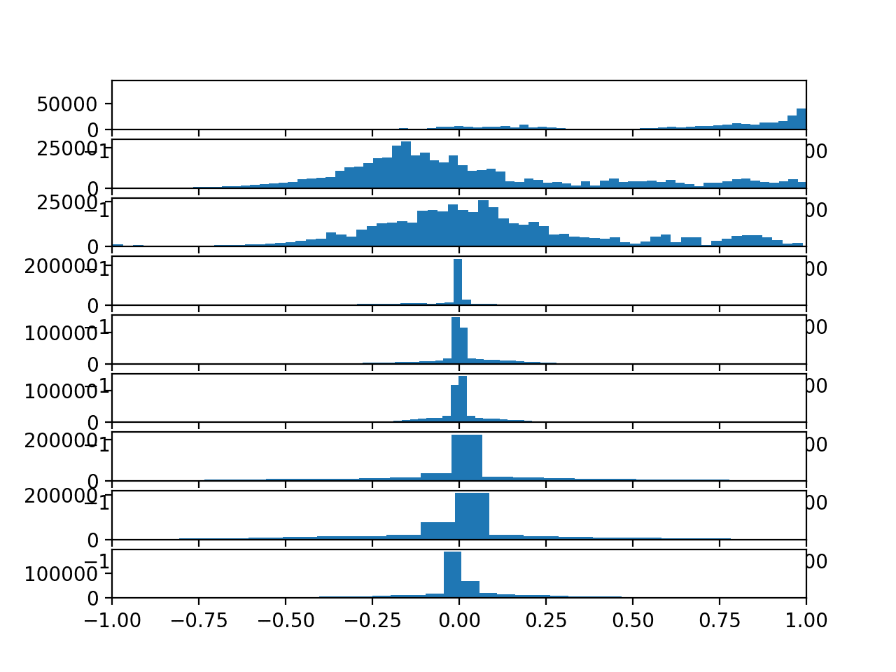
Histograms of each variable in the training data set
The data is sufficiently Gaussian-like to explore whether a standardization transform will help the model extract salient signal from the raw observations.
The function below named scale_data() can be used to standardize the data prior to fitting and evaluating the model. The StandardScaler scikit-learn class will be used to perform the transform. It is first fit on the training data (e.g. to find the mean and standard deviation for each variable), then applied to the train and test sets.
The standardization is optional, so we can apply the process and compare the results to the same code path without the standardization in a controlled experiment.
# standardize data
def scale_data(trainX, testX, standardize):
	# remove overlap
	cut = int(trainX.shape[1] / 2)
	longX = trainX[:, -cut:, :]
	# flatten windows
	longX = longX.reshape((longX.shape[0] * longX.shape[1], longX.shape[2]))
	# flatten train and test
	flatTrainX = trainX.reshape((trainX.shape[0] * trainX.shape[1], trainX.shape[2]))
	flatTestX = testX.reshape((testX.shape[0] * testX.shape[1], testX.shape[2]))
	# standardize
	if standardize:
		s = StandardScaler()
		# fit on training data
		s.fit(longX)
		# apply to training and test data
		longX = s.transform(longX)
		flatTrainX = s.transform(flatTrainX)
		flatTestX = s.transform(flatTestX)
	# reshape
	flatTrainX = flatTrainX.reshape((trainX.shape))
	flatTestX = flatTestX.reshape((testX.shape))
	return flatTrainX, flatTestX
We can update the evaluate_model() function to take a parameter, then use this parameter to decide whether or not to perform the standardization.
# fit and evaluate a model
def evaluate_model(trainX, trainy, testX, testy, param):
	verbose, epochs, batch_size = 0, 10, 32
	n_timesteps, n_features, n_outputs = trainX.shape[1], trainX.shape[2], trainy.shape[1]
	# scale data
	trainX, testX = scale_data(trainX, testX, param)
	model = Sequential()
	model.add(Conv1D(filters=64, kernel_size=3, activation='relu', input_shape=(n_timesteps,n_features)))
	model.add(Conv1D(filters=64, kernel_size=3, activation='relu'))
	model.add(Dropout(0.5))
	model.add(MaxPooling1D(pool_size=2))
	model.add(Flatten())
	model.add(Dense(100, activation='relu'))
	model.add(Dense(n_outputs, activation='softmax'))
	model.compile(loss='categorical_crossentropy', optimizer='adam', metrics=['accuracy'])
	# fit network
	model.fit(trainX, trainy, epochs=epochs, batch_size=batch_size, verbose=verbose)
	# evaluate model
	_, accuracy = model.evaluate(testX, testy, batch_size=batch_size, verbose=0)
	return accuracy
We can also update the run_experiment() to repeat the experiment 10 times for each parameter; in this case, only two parameters will be evaluated [False, True] for no standardization and standardization respectively.
# run an experiment
def run_experiment(params, repeats=10):
	# load data
	trainX, trainy, testX, testy = load_dataset()
	# test each parameter
	all_scores = list()
	for p in params:
		# repeat experiment
		scores = list()
		for r in range(repeats):
			score = evaluate_model(trainX, trainy, testX, testy, p)
			score = score * 100.0
			print('>p=%d #%d: %.3f' % (p, r+1, score))
			scores.append(score)
		all_scores.append(scores)
	# summarize results
	summarize_results(all_scores, params)
This will result in two samples of results that can be compared.
We will update the summarize_results() function to summarize the sample of results for each configuration parameter and to create a boxplot to compare each sample of results.
# summarize scores
def summarize_results(scores, params):
	print(scores, params)
	# summarize mean and standard deviation
	for i in range(len(scores)):
		m, s = mean(scores[i]), std(scores[i])
		print('Param=%d: %.3f%% (+/-%.3f)' % (params[i], m, s))
	# boxplot of scores
	pyplot.boxplot(scores, labels=params)
	pyplot.savefig('exp_cnn_standardize.png')
These updates will allow us to directly compare the results of a model fit as before and a model fit on the dataset after it has been standardized.
It is also a generic change that will allow us to evaluate and compare the results of other sets of parameters in the following sections.
The complete code listing is provided below.
# cnn model with standardization
from numpy import mean
from numpy import std
from numpy import dstack
from pandas import read_csv
from matplotlib import pyplot
from sklearn.preprocessing import StandardScaler
from keras.models import Sequential
from keras.layers import Dense
from keras.layers import Flatten
from keras.layers import Dropout
from keras.layers.convolutional import Conv1D
from keras.layers.convolutional import MaxPooling1D
from keras.utils import to_categorical

# load a single file as a numpy array
def load_file(filepath):
	dataframe = read_csv(filepath, header=None, delim_whitespace=True)
	return dataframe.values

# load a list of files and return as a 3d numpy array
def load_group(filenames, prefix=''):
	loaded = list()
	for name in filenames:
		data = load_file(prefix + name)
		loaded.append(data)
	# stack group so that features are the 3rd dimension
	loaded = dstack(loaded)
	return loaded

# load a dataset group, such as train or test
def load_dataset_group(group, prefix=''):
	filepath = prefix + group + '/Inertial Signals/'
	# load all 9 files as a single array
	filenames = list()
	# total acceleration
	filenames += ['total_acc_x_'+group+'.txt', 'total_acc_y_'+group+'.txt', 'total_acc_z_'+group+'.txt']
	# body acceleration
	filenames += ['body_acc_x_'+group+'.txt', 'body_acc_y_'+group+'.txt', 'body_acc_z_'+group+'.txt']
	# body gyroscope
	filenames += ['body_gyro_x_'+group+'.txt', 'body_gyro_y_'+group+'.txt', 'body_gyro_z_'+group+'.txt']
	# load input data
	X = load_group(filenames, filepath)
	# load class output
	y = load_file(prefix + group + '/y_'+group+'.txt')
	return X, y

# load the dataset, returns train and test X and y elements
def load_dataset(prefix=''):
	# load all train
	trainX, trainy = load_dataset_group('train', prefix + 'HARDataset/')
	print(trainX.shape, trainy.shape)
	# load all test
	testX, testy = load_dataset_group('test', prefix + 'HARDataset/')
	print(testX.shape, testy.shape)
	# zero-offset class values
	trainy = trainy - 1
	testy = testy - 1
	# one hot encode y
	trainy = to_categorical(trainy)
	testy = to_categorical(testy)
	print(trainX.shape, trainy.shape, testX.shape, testy.shape)
	return trainX, trainy, testX, testy

# standardize data
def scale_data(trainX, testX, standardize):
	# remove overlap
	cut = int(trainX.shape[1] / 2)
	longX = trainX[:, -cut:, :]
	# flatten windows
	longX = longX.reshape((longX.shape[0] * longX.shape[1], longX.shape[2]))
	# flatten train and test
	flatTrainX = trainX.reshape((trainX.shape[0] * trainX.shape[1], trainX.shape[2]))
	flatTestX = testX.reshape((testX.shape[0] * testX.shape[1], testX.shape[2]))
	# standardize
	if standardize:
		s = StandardScaler()
		# fit on training data
		s.fit(longX)
		# apply to training and test data
		longX = s.transform(longX)
		flatTrainX = s.transform(flatTrainX)
		flatTestX = s.transform(flatTestX)
	# reshape
	flatTrainX = flatTrainX.reshape((trainX.shape))
	flatTestX = flatTestX.reshape((testX.shape))
	return flatTrainX, flatTestX

# fit and evaluate a model
def evaluate_model(trainX, trainy, testX, testy, param):
	verbose, epochs, batch_size = 0, 10, 32
	n_timesteps, n_features, n_outputs = trainX.shape[1], trainX.shape[2], trainy.shape[1]
	# scale data
	trainX, testX = scale_data(trainX, testX, param)
	model = Sequential()
	model.add(Conv1D(filters=64, kernel_size=3, activation='relu', input_shape=(n_timesteps,n_features)))
	model.add(Conv1D(filters=64, kernel_size=3, activation='relu'))
	model.add(Dropout(0.5))
	model.add(MaxPooling1D(pool_size=2))
	model.add(Flatten())
	model.add(Dense(100, activation='relu'))
	model.add(Dense(n_outputs, activation='softmax'))
	model.compile(loss='categorical_crossentropy', optimizer='adam', metrics=['accuracy'])
	# fit network
	model.fit(trainX, trainy, epochs=epochs, batch_size=batch_size, verbose=verbose)
	# evaluate model
	_, accuracy = model.evaluate(testX, testy, batch_size=batch_size, verbose=0)
	return accuracy

# summarize scores
def summarize_results(scores, params):
	print(scores, params)
	# summarize mean and standard deviation
	for i in range(len(scores)):
		m, s = mean(scores[i]), std(scores[i])
		print('Param=%s: %.3f%% (+/-%.3f)' % (params[i], m, s))
	# boxplot of scores
	pyplot.boxplot(scores, labels=params)
	pyplot.savefig('exp_cnn_standardize.png')

# run an experiment
def run_experiment(params, repeats=10):
	# load data
	trainX, trainy, testX, testy = load_dataset()
	# test each parameter
	all_scores = list()
	for p in params:
		# repeat experiment
		scores = list()
		for r in range(repeats):
			score = evaluate_model(trainX, trainy, testX, testy, p)
			score = score * 100.0
			print('>p=%s #%d: %.3f' % (p, r+1, score))
			scores.append(score)
		all_scores.append(scores)
	# summarize results
	summarize_results(all_scores, params)

# run the experiment
n_params = [False, True]
run_experiment(n_params)
Running the example may take a few minutes, depending on your hardware.
The performance is printed for each evaluated model. At the end of the run, the performance of each of the tested configurations is summarized showing the mean and the standard deviation.
We can see that it does look like standardizing the dataset prior to modeling does result in a small lift in performance from about 90.4% accuracy (close to what we saw in the previous section) to about 91.5% accuracy.
Note: Given the stochastic nature of the algorithm, your specific results may vary.
(7352, 128, 9) (7352, 1)
(2947, 128, 9) (2947, 1)
(7352, 128, 9) (7352, 6) (2947, 128, 9) (2947, 6)

>p=False #1: 91.483
>p=False #2: 91.245
>p=False #3: 90.838
>p=False #4: 89.243
>p=False #5: 90.193
>p=False #6: 90.465
>p=False #7: 90.397
>p=False #8: 90.567
>p=False #9: 88.938
>p=False #10: 91.144
>p=True #1: 92.908
>p=True #2: 90.940
>p=True #3: 92.297
>p=True #4: 91.822
>p=True #5: 92.094
>p=True #6: 91.313
>p=True #7: 91.653
>p=True #8: 89.141
>p=True #9: 91.110
>p=True #10: 91.890

[[91.48286392941975, 91.24533423820834, 90.83814048184594, 89.24329826942655, 90.19341703427214, 90.46487953851374, 90.39701391245333, 90.56667797760434, 88.93790295215473, 91.14353579911774], [92.90804207668816, 90.93993892093654, 92.29725144214456, 91.82219205972176, 92.09365456396336, 91.31319986426874, 91.65252799457076, 89.14149983033593, 91.10960298608755, 91.89005768578215]] [False, True]

Param=False: 90.451% (+/-0.785)
Param=True: 91.517% (+/-0.965)
A box and whisker plot of the results is also created.
This allows the two samples of results to be compared in a nonparametric way, showing the median and the middle 50% of each sample.
We can see that the distribution of results with standardization is quite different from the distribution of results without standardization. This is likely a real effect.
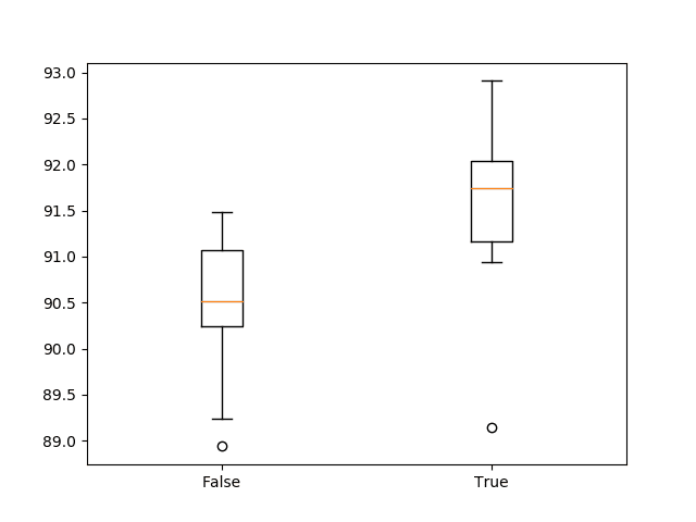
Box and whisker plot of 1D CNN with and without standardization
Number of Filters
Now that we have an experimental framework, we can explore varying other hyperparameters of the model.
An important hyperparameter for the CNN is the number of filter maps. We can experiment with a range of different values, from less to many more than the 64 used in the first model that we developed.
Specifically, we will try the following numbers of feature maps:
n_params = [8, 16, 32, 64, 128, 256]
We can use the same code from the previous section and update the evaluate_model() function to use the provided parameter as the number of filters in the Conv1D layers. We can also update the summarize_results() function to save the boxplot as exp_cnn_filters.png.
The complete code example is listed below.
# cnn model with filters
from numpy import mean
from numpy import std
from numpy import dstack
from pandas import read_csv
from matplotlib import pyplot
from keras.models import Sequential
from keras.layers import Dense
from keras.layers import Flatten
from keras.layers import Dropout
from keras.layers.convolutional import Conv1D
from keras.layers.convolutional import MaxPooling1D
from keras.utils import to_categorical

# load a single file as a numpy array
def load_file(filepath):
	dataframe = read_csv(filepath, header=None, delim_whitespace=True)
	return dataframe.values

# load a list of files and return as a 3d numpy array
def load_group(filenames, prefix=''):
	loaded = list()
	for name in filenames:
		data = load_file(prefix + name)
		loaded.append(data)
	# stack group so that features are the 3rd dimension
	loaded = dstack(loaded)
	return loaded

# load a dataset group, such as train or test
def load_dataset_group(group, prefix=''):
	filepath = prefix + group + '/Inertial Signals/'
	# load all 9 files as a single array
	filenames = list()
	# total acceleration
	filenames += ['total_acc_x_'+group+'.txt', 'total_acc_y_'+group+'.txt', 'total_acc_z_'+group+'.txt']
	# body acceleration
	filenames += ['body_acc_x_'+group+'.txt', 'body_acc_y_'+group+'.txt', 'body_acc_z_'+group+'.txt']
	# body gyroscope
	filenames += ['body_gyro_x_'+group+'.txt', 'body_gyro_y_'+group+'.txt', 'body_gyro_z_'+group+'.txt']
	# load input data
	X = load_group(filenames, filepath)
	# load class output
	y = load_file(prefix + group + '/y_'+group+'.txt')
	return X, y

# load the dataset, returns train and test X and y elements
def load_dataset(prefix=''):
	# load all train
	trainX, trainy = load_dataset_group('train', prefix + 'HARDataset/')
	print(trainX.shape, trainy.shape)
	# load all test
	testX, testy = load_dataset_group('test', prefix + 'HARDataset/')
	print(testX.shape, testy.shape)
	# zero-offset class values
	trainy = trainy - 1
	testy = testy - 1
	# one hot encode y
	trainy = to_categorical(trainy)
	testy = to_categorical(testy)
	print(trainX.shape, trainy.shape, testX.shape, testy.shape)
	return trainX, trainy, testX, testy

# fit and evaluate a model
def evaluate_model(trainX, trainy, testX, testy, n_filters):
	verbose, epochs, batch_size = 0, 10, 32
	n_timesteps, n_features, n_outputs = trainX.shape[1], trainX.shape[2], trainy.shape[1]
	model = Sequential()
	model.add(Conv1D(filters=n_filters, kernel_size=3, activation='relu', input_shape=(n_timesteps,n_features)))
	model.add(Conv1D(filters=n_filters, kernel_size=3, activation='relu'))
	model.add(Dropout(0.5))
	model.add(MaxPooling1D(pool_size=2))
	model.add(Flatten())
	model.add(Dense(100, activation='relu'))
	model.add(Dense(n_outputs, activation='softmax'))
	model.compile(loss='categorical_crossentropy', optimizer='adam', metrics=['accuracy'])
	# fit network
	model.fit(trainX, trainy, epochs=epochs, batch_size=batch_size, verbose=verbose)
	# evaluate model
	_, accuracy = model.evaluate(testX, testy, batch_size=batch_size, verbose=0)
	return accuracy

# summarize scores
def summarize_results(scores, params):
	print(scores, params)
	# summarize mean and standard deviation
	for i in range(len(scores)):
		m, s = mean(scores[i]), std(scores[i])
		print('Param=%d: %.3f%% (+/-%.3f)' % (params[i], m, s))
	# boxplot of scores
	pyplot.boxplot(scores, labels=params)
	pyplot.savefig('exp_cnn_filters.png')

# run an experiment
def run_experiment(params, repeats=10):
	# load data
	trainX, trainy, testX, testy = load_dataset()
	# test each parameter
	all_scores = list()
	for p in params:
		# repeat experiment
		scores = list()
		for r in range(repeats):
			score = evaluate_model(trainX, trainy, testX, testy, p)
			score = score * 100.0
			print('>p=%d #%d: %.3f' % (p, r+1, score))
			scores.append(score)
		all_scores.append(scores)
	# summarize results
	summarize_results(all_scores, params)

# run the experiment
n_params = [8, 16, 32, 64, 128, 256]
run_experiment(n_params)
Running the example repeats the experiment for each of the specified number of filters.
At the end of the run, a summary of the results with each number of filters is presented.
We can see perhaps a trend of increasing average performance with the increase in the number of filter maps. The variance stays pretty constant, and perhaps 128 feature maps might be a good configuration for the network.
...
Param=8: 89.148% (+/-0.790)
Param=16: 90.383% (+/-0.613)
Param=32: 90.356% (+/-1.039)
Param=64: 90.098% (+/-0.615)
Param=128: 91.032% (+/-0.702)
Param=256: 90.706% (+/-0.997)
A box and whisker plot of the results is also created, allowing the distribution of results with each number of filters to be compared.
From the plot, we can see the trend upward in terms of median classification accuracy (orange line on the box) with the increase in the number of feature maps. We do see a dip at 64 feature maps (the default or baseline in our experiments), which is surprising, and perhaps a plateau in accuracy across 32, 128, and 256 filter maps. Perhaps 32 would be a more stable configuration.
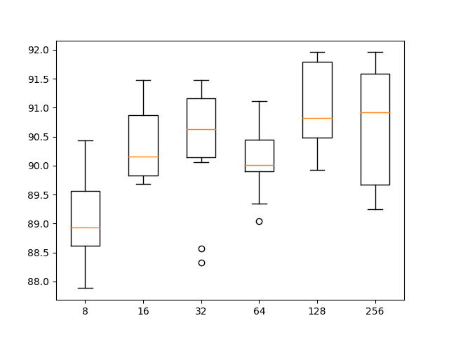
Box and whisker plot of 1D CNN with different numbers of filter maps
Size of Kernel
The size of the kernel is another important hyperparameter of the 1D CNN to tune.
The kernel size controls the number of time steps consider in each “read” of the input sequence, that is then projected onto the feature map (via the convolutional process).
A large kernel size means a less rigorous reading of the data, but may result in a more generalized snapshot of the input.
We can use the same experimental set-up and test a suite of different kernel sizes in addition to the default of three time steps. The full list of values is as follows:
n_params = [2, 3, 5, 7, 11]
The complete code listing is provided below:
# cnn model vary kernel size
from numpy import mean
from numpy import std
from numpy import dstack
from pandas import read_csv
from matplotlib import pyplot
from keras.models import Sequential
from keras.layers import Dense
from keras.layers import Flatten
from keras.layers import Dropout
from keras.layers.convolutional import Conv1D
from keras.layers.convolutional import MaxPooling1D
from keras.utils import to_categorical

# load a single file as a numpy array
def load_file(filepath):
	dataframe = read_csv(filepath, header=None, delim_whitespace=True)
	return dataframe.values

# load a list of files and return as a 3d numpy array
def load_group(filenames, prefix=''):
	loaded = list()
	for name in filenames:
		data = load_file(prefix + name)
		loaded.append(data)
	# stack group so that features are the 3rd dimension
	loaded = dstack(loaded)
	return loaded

# load a dataset group, such as train or test
def load_dataset_group(group, prefix=''):
	filepath = prefix + group + '/Inertial Signals/'
	# load all 9 files as a single array
	filenames = list()
	# total acceleration
	filenames += ['total_acc_x_'+group+'.txt', 'total_acc_y_'+group+'.txt', 'total_acc_z_'+group+'.txt']
	# body acceleration
	filenames += ['body_acc_x_'+group+'.txt', 'body_acc_y_'+group+'.txt', 'body_acc_z_'+group+'.txt']
	# body gyroscope
	filenames += ['body_gyro_x_'+group+'.txt', 'body_gyro_y_'+group+'.txt', 'body_gyro_z_'+group+'.txt']
	# load input data
	X = load_group(filenames, filepath)
	# load class output
	y = load_file(prefix + group + '/y_'+group+'.txt')
	return X, y

# load the dataset, returns train and test X and y elements
def load_dataset(prefix=''):
	# load all train
	trainX, trainy = load_dataset_group('train', prefix + 'HARDataset/')
	print(trainX.shape, trainy.shape)
	# load all test
	testX, testy = load_dataset_group('test', prefix + 'HARDataset/')
	print(testX.shape, testy.shape)
	# zero-offset class values
	trainy = trainy - 1
	testy = testy - 1
	# one hot encode y
	trainy = to_categorical(trainy)
	testy = to_categorical(testy)
	print(trainX.shape, trainy.shape, testX.shape, testy.shape)
	return trainX, trainy, testX, testy

# fit and evaluate a model
def evaluate_model(trainX, trainy, testX, testy, n_kernel):
	verbose, epochs, batch_size = 0, 15, 32
	n_timesteps, n_features, n_outputs = trainX.shape[1], trainX.shape[2], trainy.shape[1]
	model = Sequential()
	model.add(Conv1D(filters=64, kernel_size=n_kernel, activation='relu', input_shape=(n_timesteps,n_features)))
	model.add(Conv1D(filters=64, kernel_size=n_kernel, activation='relu'))
	model.add(Dropout(0.5))
	model.add(MaxPooling1D(pool_size=2))
	model.add(Flatten())
	model.add(Dense(100, activation='relu'))
	model.add(Dense(n_outputs, activation='softmax'))
	model.compile(loss='categorical_crossentropy', optimizer='adam', metrics=['accuracy'])
	# fit network
	model.fit(trainX, trainy, epochs=epochs, batch_size=batch_size, verbose=verbose)
	# evaluate model
	_, accuracy = model.evaluate(testX, testy, batch_size=batch_size, verbose=0)
	return accuracy

# summarize scores
def summarize_results(scores, params):
	print(scores, params)
	# summarize mean and standard deviation
	for i in range(len(scores)):
		m, s = mean(scores[i]), std(scores[i])
		print('Param=%d: %.3f%% (+/-%.3f)' % (params[i], m, s))
	# boxplot of scores
	pyplot.boxplot(scores, labels=params)
	pyplot.savefig('exp_cnn_kernel.png')

# run an experiment
def run_experiment(params, repeats=10):
	# load data
	trainX, trainy, testX, testy = load_dataset()
	# test each parameter
	all_scores = list()
	for p in params:
		# repeat experiment
		scores = list()
		for r in range(repeats):
			score = evaluate_model(trainX, trainy, testX, testy, p)
			score = score * 100.0
			print('>p=%d #%d: %.3f' % (p, r+1, score))
			scores.append(score)
		all_scores.append(scores)
	# summarize results
	summarize_results(all_scores, params)

# run the experiment
n_params = [2, 3, 5, 7, 11]
run_experiment(n_params)
Running the example tests each kernel size in turn.
The results are summarized at the end of the run. We can see a general increase in model performance with the increase in kernel size.
The results suggest a kernel size of 5 might be good with a mean skill of about 91.8%, but perhaps a size of 7 or 11 may also be just as good with a smaller standard deviation.
...
Param=2: 90.176% (+/-0.724)
Param=3: 90.275% (+/-1.277)
Param=5: 91.853% (+/-1.249)
Param=7: 91.347% (+/-0.852)
Param=11: 91.456% (+/-0.743)
A box and whisker plot of the results is also created.
The results suggest that a larger kernel size does appear to result in better accuracy and that perhaps a kernel size of 7 provides a good balance between good performance and low variance.
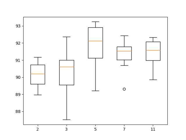
Box and whisker plot of 1D CNN with different numbers of kernel sizes
This is just the beginning of tuning the model, although we have focused on perhaps the more important elements. It might be interesting to explore combinations of some of the above findings to see if performance can be lifted even further.
It may also be interesting to increase the number of repeats from 10 to 30 or more to see if it results in more stable findings.
Multi-Headed Convolutional Neural Network
Another popular approach with CNNs is to have a multi-headed model, where each head of the model reads the input time steps using a different sized kernel.
For example, a three-headed model may have three different kernel sizes of 3, 5, 11, allowing the model to read and interpret the sequence data at three different resolutions. The interpretations from all three heads are then concatenated within the model and interpreted by a fully-connected layer before a prediction is made.
We can implement a multi-headed 1D CNN using the Keras functional API. For a gentle introduction to this API, see the post:
The updated version of the evaluate_model() function is listed below that creates a three-headed CNN model.
We can see that each head of the model is the same structure, although the kernel size is varied. The three heads then feed into a single merge layer before being interpreted prior to making a prediction.
# fit and evaluate a model
def evaluate_model(trainX, trainy, testX, testy):
	verbose, epochs, batch_size = 0, 10, 32
	n_timesteps, n_features, n_outputs = trainX.shape[1], trainX.shape[2], trainy.shape[1]
 	# head 1
	inputs1 = Input(shape=(n_timesteps,n_features))
	conv1 = Conv1D(filters=64, kernel_size=3, activation='relu')(inputs1)
	drop1 = Dropout(0.5)(conv1)
	pool1 = MaxPooling1D(pool_size=2)(drop1)
	flat1 = Flatten()(pool1)
	# head 2
	inputs2 = Input(shape=(n_timesteps,n_features))
	conv2 = Conv1D(filters=64, kernel_size=5, activation='relu')(inputs2)
	drop2 = Dropout(0.5)(conv2)
	pool2 = MaxPooling1D(pool_size=2)(drop2)
	flat2 = Flatten()(pool2)
	# head 3
	inputs3 = Input(shape=(n_timesteps,n_features))
	conv3 = Conv1D(filters=64, kernel_size=11, activation='relu')(inputs3)
	drop3 = Dropout(0.5)(conv3)
	pool3 = MaxPooling1D(pool_size=2)(drop3)
	flat3 = Flatten()(pool3)
	# merge
	merged = concatenate([flat1, flat2, flat3])
	# interpretation
	dense1 = Dense(100, activation='relu')(merged)
	outputs = Dense(n_outputs, activation='softmax')(dense1)
	model = Model(inputs=[inputs1, inputs2, inputs3], outputs=outputs)
	# save a plot of the model
	plot_model(model, show_shapes=True, to_file='multichannel.png')
	model.compile(loss='categorical_crossentropy', optimizer='adam', metrics=['accuracy'])
	# fit network
	model.fit([trainX,trainX,trainX], trainy, epochs=epochs, batch_size=batch_size, verbose=verbose)
	# evaluate model
	_, accuracy = model.evaluate([testX,testX,testX], testy, batch_size=batch_size, verbose=0)
	return accuracy
When the model is created, a plot of the network architecture is created; provided below, it gives a clear idea of how the constructed model fits together.
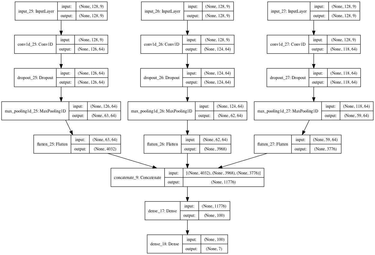
Plot of the Multi-Headed 1D Convolutional Neural Network
Other aspects of the model could be varied across the heads, such as the number of filters or even the preparation of the data itself.
The complete code example with the multi-headed 1D CNN is listed below.
# multi-headed cnn model
from numpy import mean
from numpy import std
from numpy import dstack
from pandas import read_csv
from matplotlib import pyplot
from keras.utils import to_categorical
from keras.utils.vis_utils import plot_model
from keras.models import Model
from keras.layers import Input
from keras.layers import Dense
from keras.layers import Flatten
from keras.layers import Dropout
from keras.layers.convolutional import Conv1D
from keras.layers.convolutional import MaxPooling1D
from keras.layers.merge import concatenate

# load a single file as a numpy array
def load_file(filepath):
	dataframe = read_csv(filepath, header=None, delim_whitespace=True)
	return dataframe.values

# load a list of files and return as a 3d numpy array
def load_group(filenames, prefix=''):
	loaded = list()
	for name in filenames:
		data = load_file(prefix + name)
		loaded.append(data)
	# stack group so that features are the 3rd dimension
	loaded = dstack(loaded)
	return loaded

# load a dataset group, such as train or test
def load_dataset_group(group, prefix=''):
	filepath = prefix + group + '/Inertial Signals/'
	# load all 9 files as a single array
	filenames = list()
	# total acceleration
	filenames += ['total_acc_x_'+group+'.txt', 'total_acc_y_'+group+'.txt', 'total_acc_z_'+group+'.txt']
	# body acceleration
	filenames += ['body_acc_x_'+group+'.txt', 'body_acc_y_'+group+'.txt', 'body_acc_z_'+group+'.txt']
	# body gyroscope
	filenames += ['body_gyro_x_'+group+'.txt', 'body_gyro_y_'+group+'.txt', 'body_gyro_z_'+group+'.txt']
	# load input data
	X = load_group(filenames, filepath)
	# load class output
	y = load_file(prefix + group + '/y_'+group+'.txt')
	return X, y

# load the dataset, returns train and test X and y elements
def load_dataset(prefix=''):
	# load all train
	trainX, trainy = load_dataset_group('train', prefix + 'HARDataset/')
	print(trainX.shape, trainy.shape)
	# load all test
	testX, testy = load_dataset_group('test', prefix + 'HARDataset/')
	print(testX.shape, testy.shape)
	# zero-offset class values
	trainy = trainy - 1
	testy = testy - 1
	# one hot encode y
	trainy = to_categorical(trainy)
	testy = to_categorical(testy)
	print(trainX.shape, trainy.shape, testX.shape, testy.shape)
	return trainX, trainy, testX, testy

# fit and evaluate a model
def evaluate_model(trainX, trainy, testX, testy):
	verbose, epochs, batch_size = 0, 10, 32
	n_timesteps, n_features, n_outputs = trainX.shape[1], trainX.shape[2], trainy.shape[1]
 	# head 1
	inputs1 = Input(shape=(n_timesteps,n_features))
	conv1 = Conv1D(filters=64, kernel_size=3, activation='relu')(inputs1)
	drop1 = Dropout(0.5)(conv1)
	pool1 = MaxPooling1D(pool_size=2)(drop1)
	flat1 = Flatten()(pool1)
	# head 2
	inputs2 = Input(shape=(n_timesteps,n_features))
	conv2 = Conv1D(filters=64, kernel_size=5, activation='relu')(inputs2)
	drop2 = Dropout(0.5)(conv2)
	pool2 = MaxPooling1D(pool_size=2)(drop2)
	flat2 = Flatten()(pool2)
	# head 3
	inputs3 = Input(shape=(n_timesteps,n_features))
	conv3 = Conv1D(filters=64, kernel_size=11, activation='relu')(inputs3)
	drop3 = Dropout(0.5)(conv3)
	pool3 = MaxPooling1D(pool_size=2)(drop3)
	flat3 = Flatten()(pool3)
	# merge
	merged = concatenate([flat1, flat2, flat3])
	# interpretation
	dense1 = Dense(100, activation='relu')(merged)
	outputs = Dense(n_outputs, activation='softmax')(dense1)
	model = Model(inputs=[inputs1, inputs2, inputs3], outputs=outputs)
	# save a plot of the model
	plot_model(model, show_shapes=True, to_file='multichannel.png')
	model.compile(loss='categorical_crossentropy', optimizer='adam', metrics=['accuracy'])
	# fit network
	model.fit([trainX,trainX,trainX], trainy, epochs=epochs, batch_size=batch_size, verbose=verbose)
	# evaluate model
	_, accuracy = model.evaluate([testX,testX,testX], testy, batch_size=batch_size, verbose=0)
	return accuracy

# summarize scores
def summarize_results(scores):
	print(scores)
	m, s = mean(scores), std(scores)
	print('Accuracy: %.3f%% (+/-%.3f)' % (m, s))

# run an experiment
def run_experiment(repeats=10):
	# load data
	trainX, trainy, testX, testy = load_dataset()
	# repeat experiment
	scores = list()
	for r in range(repeats):
		score = evaluate_model(trainX, trainy, testX, testy)
		score = score * 100.0
		print('>#%d: %.3f' % (r+1, score))
		scores.append(score)
	# summarize results
	summarize_results(scores)

# run the experiment
run_experiment()
Running the example prints the performance of the model each repeat of the experiment and then summarizes the estimated score as the mean and standard deviation, as we did in the first case with the simple 1D CNN.
We can see that the average performance of the model is about 91.6% classification accuracy with a standard deviation of about 0.8.
This example may be used as the basis for exploring a variety of other models that vary different model hyperparameters and even different data preparation schemes across the input heads.
It would not be an apples-to-apples comparison to compare this result with a single-headed CNN given the relative tripling of the resources in this model. Perhaps an apples-to-apples comparison would be a model with the same architecture and the same number of filters across each input head of the model.
>#1: 91.788
>#2: 92.942
>#3: 91.551
>#4: 91.415
>#5: 90.974
>#6: 91.992
>#7: 92.162
>#8: 89.888
>#9: 92.671
>#10: 91.415

[91.78825924669155, 92.94197488971835, 91.55072955548015, 91.41499830335935, 90.97387173396675, 91.99185612487275, 92.16152019002375, 89.88802171700034, 92.67051238547675, 91.41499830335935]

Accuracy: 91.680% (+/-0.823)
Extensions
This section lists some ideas for extending the tutorial that you may wish to explore.
- Date Preparation. Explore other data preparation schemes such as data normalization and perhaps normalization after standardization.
- Network Architecture. Explore other network architectures, such as deeper CNN architectures and deeper fully-connected layers for interpreting the CNN input features.
- Diagnostics. Use simple learning curve diagnostics to interpret how the model is learning over the epochs and whether more regularization, different learning rates, or different batch sizes or numbers of epochs may result in a better performing or more stable model.
If you explore any of these extensions, I’d love to know.
Further Reading
This section provides more resources on the topic if you are looking to go deeper.
Papers
- A Public Domain Dataset for Human Activity Recognition Using Smartphones, 2013.
- Human Activity Recognition on Smartphones using a Multiclass Hardware-Friendly Support Vector Machine, 2012.
Articles
- Human Activity Recognition Using Smartphones Data Set, UCI Machine Learning Repository
- Activity recognition, Wikipedia
- Activity Recognition Experiment Using Smartphone Sensors, Video.
Summary
In this tutorial, you discovered how to develop one-dimensional convolutional neural networks for time series classification on the problem of human activity recognition.
Specifically, you learned:
- How to load and prepare the data for a standard human activity recognition dataset and develop a single 1D CNN model that achieves excellent performance on the raw data.
- How to further tune the performance of the model, including data transformation, filter maps, and kernel sizes.
- How to develop a sophisticated multi-headed one-dimensional convolutional neural network model that provides an ensemble-like result.
Do you have any questions?
Ask your questions in the comments below and I will do my best to answer.
The post How to Develop 1D Convolutional Neural Network Models for Human Activity Recognition appeared first on Machine Learning Mastery.