Author: Burak Himmetoglu
Introduction
Feature selection and engineering are the most important factors which affect the success of predictive modeling. This remains true even today despite the success of deep learning, which comes with automatic feature engineering. Parsimonious and interpretable models provide simple insights into business problems and therefore they are deemed very valuable. Furthermore, in many occasions the underlying size and structure of the data being analyzed may not allow the use of complex models that have many parameters to tune. For example, in clinical settings where the number of samples is usually much lower than the number of features one could extract (e.g. gene expression studies, patient specific physiologic data etc.), simpler models are preferable. These high dimensional problems pose significant challenges, and numerous techniques have been developed over the years to provide solutions. In this post, I will review a few of the common methods and illustrate their use in some sample cases. I will focus on binary classification problems for simplicity.
I will use two datasets for the discussion in the post:
- Synthetic datasets (using scikit-learn’s make_classification utility)
- The LSVT dataset from UCI repository
I posted the Python code and several notebooks in a Github repository for interested readers.
Visual exploration of data
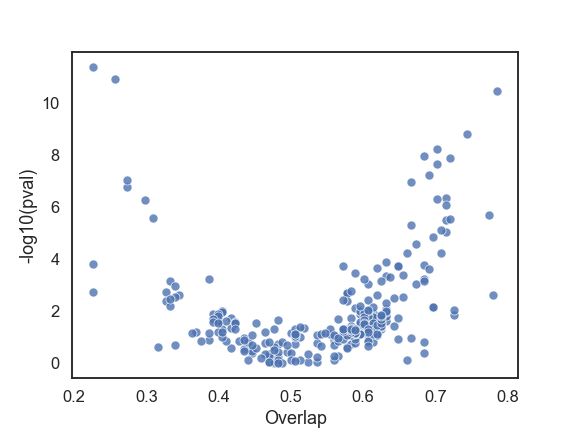
Visual exploration of the dataset is the first and possibly the most crucial stage of any model building effort. There are numerous online articles one can find about data exploration and majority of them are mostly focused on visualizing one or a few features at a time. While an analysis of one/few feature(s) at a time is very valuable, when one is faced with the task of selecting features from a large pool, it can become quite daunting. In case of binary classification problems, a simple scatter plot with one axis displaying statistical significance and the other an effect size proves to be quite useful (e.g. volcano plots). The figure below is an example of such visualization, where the y-axis is the negative log of the p-value for the t-test, and the x-axis is the overlap (defined below) for each feature.
P-value and overlap for each feature in the LSVT dataset
The scatter plot is constructed from the LSVT dataset, which will be discussed in a bit more detail below. The overlap represents the misclassification rate in the distribution of a single feature, therefore lower values are better. To compute the overlap, first a weighted average of the means of features for each binary (+/-) class are computed. The fraction of (+) observations below the average and the (-) observations above the average result in the overlap value (see figure below). Therefore in the above scatter plot, the features that fall in the top left corner are the best features. Majority of the features have high overlap and are statistically insignificant when used alone. Notice also that there are features with very small p-values but high overlap (top right). This is one of the reasons why p-values alone could be misleading.
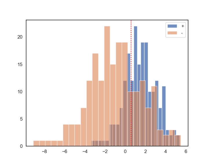 The red vertical dotted line is the weighted average of the means of + and – classes. Higher overlap corresponds to a case when the + and – distributions are close to each other
This initial exploration provides us with information about which features we would expect to be important in our modeling efforts. After this step, we can delve into the details of how one can systematically choose the features for best performance. In this rest of the post, I will present several approaches to achieve this goal.
Ridge Regression and LASSO
These linear models are extremely useful for many problems and they have mechanisms to implicitly (ridge) and explicitly (LASSO) reduce the number of features. In the binary classification setting, these methods are simple extensions of logistic regression by an addition of a regularization term. Ridge regression uses sum of squares of feature weights, while LASSO uses sum of absolute values of feature weights as the regularization term. The regularization term shrinks feature weights (with respect to a fit with no regularization), lowering the effective degrees of freedom. LASSO can shrink the weights of features exactly to zero, resulting in explicit feature selection.
 Ridge (left) and LASSO (right) regression feature weight shrinkage
The above figure illustrates, for a synthetic classification problem with 75 features, how LASSO and Ridge regression differ in shrinking feature weights. The regularization parameter (C) controls the number of chosen features, which can be determined by cross-validation. Feature selection by LASSO is automatically achieved by simply training it. After training, the LASSO model has only 21 features with nonzero weights (red dotted line in the above figure indicates the tuned value for hyperparameter C). Instead, Ridge regression keeps all the features, but shrinks their weights close to zero, implicitly reducing the effective number of features.
It is also possible to have both LASSO and Ridge regularization terms in a single model (glmnet), leveraging the advantages of both methods. When there are many correlated features, LASSO tends to pick one of them at random and shrinks the rest to zero. Instead, Ridge regression tends to shrink weights of correlated features towards the same value. In these cases, a combination of two regularization terms can be advantageous.
Note: I referenced scikit-learn’s implementation of LASSO and Ridge regression where the hyper-parameter (C) is a prefactor in the loss term, similar to the case of SVMs. The traditional implementations have the hyperparameter (lambda) in front of the shrinkage term, and they are related to scikit-learn’s simply by C = 1/lambda.
Stepwise Feature Selection
As the name suggests, these methods select features in steps based on a specified performance criteria. Methods such as forward and backward feature selection are quite well-known and a nice discussion of them can be found in Introduction to Statistical Learning (ISLR). Currently, scikit-learn has an implementation of a kind of backward selection method, recursive feature elimination (RFE). Since my discussion here is more focused towards large dimensional datasets, I will discuss the forward selection method. Forward selection starts with one feature and recursively adds more to the model until a user specified criterion is achieved. While RFE works for large dimensional datasets, one may end up with a final model which still has many features.
Traditional feature selection implementations use metrics such as adjusted R-squared and AIC to determine the number of features (see ISLR). Instead, I will consider cross-validation (CV) based performance metrics as the means to pick the best features. The strategy is to optimize hyper-parameters and features together using CV. As an example, consider the case where we want to forward select the features to use in a ridge regression model. Then, we will have to perform a search in the feature x hyperparameter space. The pseudo-code for this procedure is shown below:
 Pseudo-code forward feature selection algorithm
The performance metric (in our case, the negative log loss), starts at a low value with a single feature model and reaches a large enough value where the algorithm can stop. For the synthetic dataset with 75 total features, a maximal CV score is reached at 28 features, as shown below.
 Forward feature selection procedure. The desired number of features is obtained when CV score is maximized (red dotted line)
The forward selection procedure will yield a parsimonious model with the best CV performance. While this method uses out-of-sample scores to reduce possible overfitting problems in choosing features, care must be taken when the number of samples is smaller than the number of features (e.g. LSVT dataset). In this case, the algorithm may choose a representation of data based on a few features, which may turn out to be sub-optimal for an unseen test data. In such cases, Ridge regression may lead to better results, since all features are included with an implicit dimensional reduction (see the discussion on the LSVT dataset).
Ensemble of Trees and Feature Importance
Ensemble of trees (e.g. random forest, boosting) are powerful and popular algorithms. While one can simply decide to employ these models directly, there are two caveats to their use:
- They are complex models and not easy to interpret.
- Extra care must be taken in training them, since they have high variance and overfitting can be difficult to mitigate (especially when the number of features exceed the number of samples).
On the other hand, they provide a simple importance measure, which can be used for feature selection. Let’s summarize how feature importances are computed:
Each decision tree is grown on a randomly selected feature set, which ranks the features according to how much they contribute to reducing misclassification (usually, Gini coefficient is used). After many trees are grown, each feature ends up with a mean (across trees) importance measure.
Feature selection can then be achieved by removing features that have importance measures smaller than a pre-specified cut-off (e.g. mean of all the feature importances). As a result, it is possible to use a tree ensemble as a filtering tool. After filtering, the selected features can be used in a simple model, such as ridge regression. Scikit-learn has a useful wrapper to use for such a procedure.
There are various issues that could arise in the approach discussed above, most of which I will not discuss in this post. Among them is the problem of setting the hyperparameters of the tree ensemble model. I simply used the tree model as a filter and did not determine its hyperparameters by CV. Empirically, I have not seen this cause problems, but it is not clear whether such a simple filtering may always work. In addition, problems may arise when there are many correlated features. In this case, a tree ensemble may filter out a good feature, since another feature (correlated to the one in question) could have already been chosen. In light of these observations, I recommend the reader to take the results from this approach with a grain of salt, and make sure to perform several tests before employing this idea in a real problem.
Comparison
Let’s compare how these feature selection methods perform for a synthetic dataset. In the table below, I show results for two versions of the synthetic data. Both have 75 features, but the first one has only 25 and the second one has only 5 informative features.
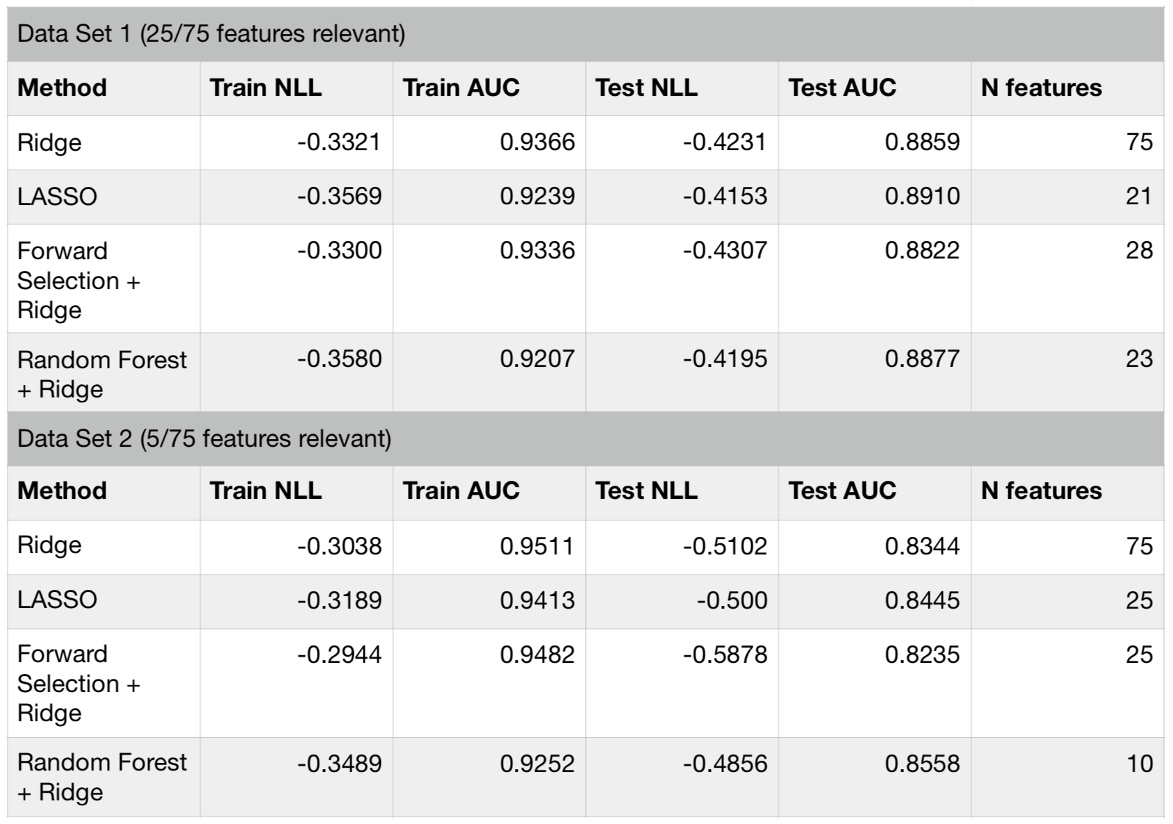 Comparison of performance metric for the two synthetic datasets
The performance of all the methods have been similar for these datasets. Below is a plot showing the resulting feature weights (rescaled) for each model. With the exception of random forest feature selector, all the methods assign high weights to roughly the same features. I do not have a clear explanation to why random forest picks different features. One the other hand, this effect can be exploited for increasing predictive performance. Since random forest features result in quite a different model with similar performance to other linear selectors (like LASSO), one can stack or blend them to achieve even better performance (see a post about stacking models here).
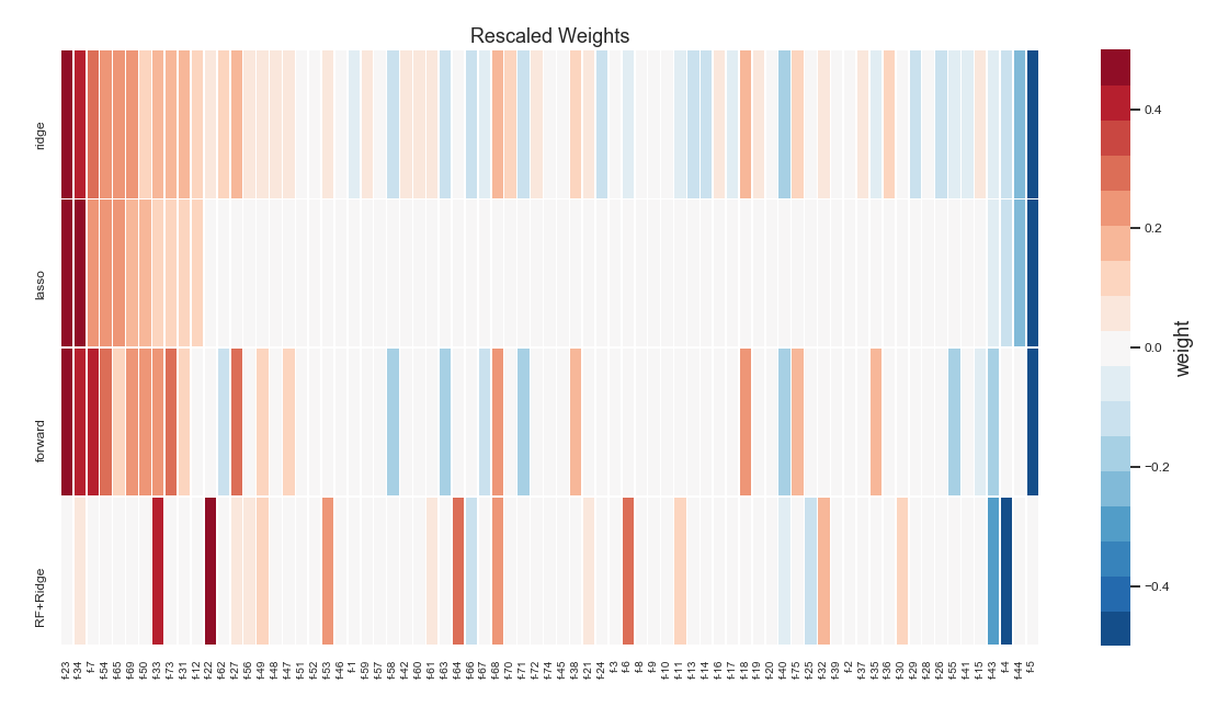 Feature weights (rescaled) from each selection algorithm
Case Study
Finally, let’s consider a real world dataset (LSVT) where the number of features is larger than the available number of observations. The dataset is composed of 310 manually engineered features from vocal recordings of patients with Parkinson’s disease. Speech experts labeled each recording as acceptable or unacceptable to assess the patients speech vocal performance degradation. The aim is to predict the assessments made by experts using a classification algorithm. Since this is a high dimensional problem (number of observations = 126), utmost care must be taken to prevent overfitting. I first divided the data into a training (70%) and test set (30%), and applied the above feature selection methods using the training set only. Then, the test set is used to assess the performance of each method. Below is a table summarizing the results:
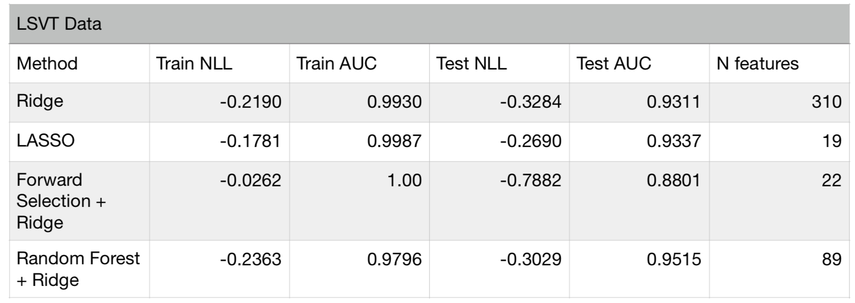 Results of feature selection methods for LSVT data
The above table shows that all models except forward selection, have similar performance. The forward selection method overfits, since it yields almost perfect score in the training set, but a much lower one on the test set. Although we used out-of-sample scores in forward selection to prevent overfitting, the small number of data instances (84 in training set) has led the algorithm to fall into the trap of selection bias (in feature space). It is therefore critical to test each feature selection approach carefully before deciding to use a final model.
In the publication where the data originates from, the whole dataset was used in training and cross-validation scores were reported as the performance measure. While this could be fine, there is always value in having an unseen part of the data for verification. If we did not have the test set, we could have concluded that the forward selection method provides the perfect answer.
References and Further Reading
There are a few resources that I find very useful and recommend interested readers to refer to for further details and methodologies.
- Introduction to Statistical Learning: A goto reference for any topic at the beginner’s level
- Elements of Statistical Learning: A more advanced and extended treatment of topics covered in ISLR
- Applied predictive modeling: An excellent resource with worked examples on some interesting datasets
- Feature Engineering and Selection: A practical approach for predictive models: Another excellent resource dedicated to feature engineering
- Github Repository accompanying this post for notebooks and code
The original blog post was posted in the author’s site.