
Author: Jason Brownlee
Grid searching is generally not an operation that we can perform with deep learning methods.
This is because deep learning methods often require large amounts of data and large models, together resulting in models that take hours, days, or weeks to train.
In those cases where the datasets are smaller, such as univariate time series, it may be possible to use a grid search to tune the hyperparameters of a deep learning model.
In this tutorial, you will discover how to develop a framework to grid search hyperparameters for deep learning models.
After completing this tutorial, you will know:
- How to develop a generic grid searching framework for tuning model hyperparameters.
- How to grid search hyperparameters for a Multilayer Perceptron model on the airline passengers univariate time series forecasting problem.
- How to adapt the framework to grid search hyperparameters for convolutional and long short-term memory neural networks.
Let’s get started.

How to Grid Search Deep Learning Models for Time Series Forecasting
Photo by Hannes Flo, some rights reserved.
Tutorial Overview
This tutorial is divided into five parts; they are:
- Time Series Problem
- Grid Search Framework
- Grid Search Multilayer Perceptron
- Grid Search Convolutional Neural Network
- Grid Search Long Short-Term Memory Network
Time Series Problem
The ‘monthly airline passenger‘ dataset summarizes the monthly total number of international passengers in thousands on for an airline from 1949 to 1960.
Download the dataset directly from here:
Save the file with the filename ‘monthly-airline-passengers.csv‘ in your current working directory.
We can load this dataset as a Pandas series using the function read_csv().
# load
series = read_csv('monthly-airline-passengers.csv', header=0, index_col=0)
Once loaded, we can summarize the shape of the dataset in order to determine the number of observations.
# summarize shape
print(series.shape)
We can then create a line plot of the series to get an idea of the structure of the series.
# plot
pyplot.plot(series)
pyplot.show()
We can tie all of this together; the complete example is listed below.
# load and plot dataset
from pandas import read_csv
from matplotlib import pyplot
# load
series = read_csv('monthly-airline-passengers.csv', header=0, index_col=0)
# summarize shape
print(series.shape)
# plot
pyplot.plot(series)
pyplot.show()
Running the example first prints the shape of the dataset.
(144, 1)
The dataset is monthly and has 12 years, or 144 observations. In our testing, we will use the last year, or 12 observations, as the test set.
A line plot is created. The dataset has an obvious trend and seasonal component. The period of the seasonal component is 12 months.
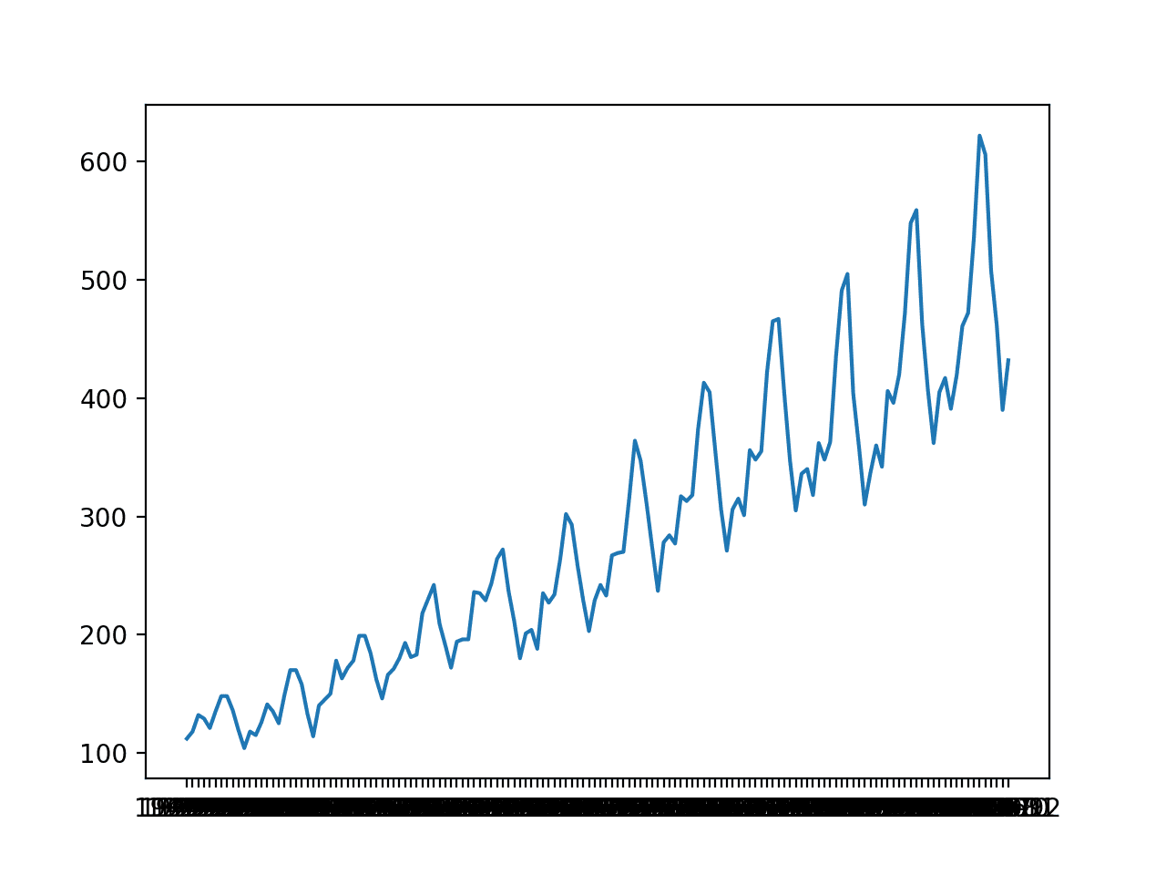
Line Plot of Monthly International Airline Passengers
In this tutorial, we will introduce the tools for grid searching, but we will not optimize the model hyperparameters for this problem. Instead, we will demonstrate how to grid search the deep learning model hyperparameters generally and find models with some skill compared to a naive model.
From prior experiments, a naive model can achieve a root mean squared error, or RMSE, of 50.70 (remember the units are thousands of passengers) by persisting the value from 12 months ago (relative index -12).
The performance of this naive model provides a bound on a model that is considered skillful for this problem. Any model that achieves a predictive performance of lower than 50.70 on the last 12 months has skill.
It should be noted that a tuned ETS model can achieve an RMSE of 17.09 and a tuned SARIMA can achieve an RMSE of 13.89. These provide a lower bound on the expectations of a well-tuned deep learning model for this problem.
Now that we have defined our problem and expectations of model skill, we can look at defining the grid search test harness.
Grid Search Framework
In this section, we will develop a grid search test harness that can be used to evaluate a range of hyperparameters for different neural network models, such as MLPs, CNNs, and LSTMs.
This section is divided into the following parts:
- Train-Test Split
- Series as Supervised Learning
- Walk-Forward Validation
- Repeat Evaluation
- Summarize Performance
- Worked Example
Train-Test Split
The first step is to split the loaded series into train and test sets.
We will use the first 11 years (132 observations) for training and the last 12 for the test set.
The train_test_split() function below will split the series taking the raw observations and the number of observations to use in the test set as arguments.
# split a univariate dataset into train/test sets
def train_test_split(data, n_test):
	return data[:-n_test], data[-n_test:]
Series as Supervised Learning
Next, we need to be able to frame the univariate series of observations as a supervised learning problem so that we can train neural network models.
A supervised learning framing of a series means that the data needs to be split into multiple examples that the model learns from and generalizes across.
Each sample must have both an input component and an output component.
The input component will be some number of prior observations, such as three years, or 36 time steps.
The output component will be the total sales in the next month because we are interested in developing a model to make one-step forecasts.
We can implement this using the shift() function on the pandas DataFrame. It allows us to shift a column down (forward in time) or back (backward in time). We can take the series as a column of data, then create multiple copies of the column, shifted forward or backward in time in order to create the samples with the input and output elements we require.
When a series is shifted down, NaN values are introduced because we don’t have values beyond the start of the series.
For example, the series defined as a column:
(t)
1
2
3
4
This column can be shifted and inserted as a column beforehand:
(t-1),		(t)
Nan,		1
1,			2
2,			3
3,			4
4			NaN
We can see that on the second row, the value 1 is provided as input as an observation at the prior time step, and 2 is the next value in the series that can be predicted, or learned by the model to be predicted when 1 is presented as input.
Rows with NaN values can be removed.
The series_to_supervised() function below implements this behavior, allowing you to specify the number of lag observations to use in the input and the number to use in the output for each sample. It will also remove rows that have NaN values as they cannot be used to train or test a model.
# transform list into supervised learning format
def series_to_supervised(data, n_in=1, n_out=1):
	df = DataFrame(data)
	cols = list()
	# input sequence (t-n, ... t-1)
	for i in range(n_in, 0, -1):
		cols.append(df.shift(i))
	# forecast sequence (t, t+1, ... t+n)
	for i in range(0, n_out):
		cols.append(df.shift(-i))
	# put it all together
	agg = concat(cols, axis=1)
	# drop rows with NaN values
	agg.dropna(inplace=True)
	return agg.values
Walk-Forward Validation
Time series forecasting models can be evaluated on a test set using walk-forward validation.
Walk-forward validation is an approach where the model makes a forecast for each observation in the test dataset one at a time. After each forecast is made for a time step in the test dataset, the true observation for the forecast is added to the test dataset and made available to the model.
Simpler models can be refit with the observation prior to making the subsequent prediction. More complex models, such as neural networks, are not refit given the much greater computational cost.
Nevertheless, the true observation for the time step can then be used as part of the input for making the prediction on the next time step.
First, the dataset is split into train and test sets. We will call the train_test_split() function to perform this split and pass in the pre-specified number of observations to use as the test data.
A model will be fit once on the training dataset for a given configuration.
We will define a generic model_fit() function to perform this operation that can be filled in for the given type of neural network that we may be interested in later. The function takes the training dataset and the model configuration and returns the fit model ready for making predictions.
# fit a model
def model_fit(train, config):
	return None
Each time step of the test dataset is enumerated. A prediction is made using the fit model.
Again, we will define a generic function named model_predict() that takes the fit model, the history, and the model configuration and makes a single one-step prediction.
# forecast with a pre-fit model
def model_predict(model, history, config):
	return 0.0
The prediction is added to a list of predictions and the true observation from the test set is added to a list of observations that was seeded with all observations from the training dataset. This list is built up during each step in the walk-forward validation, allowing the model to make a one-step prediction using the most recent history.
All of the predictions can then be compared to the true values in the test set and an error measure calculated.
We will calculate the root mean squared error, or RMSE, between predictions and the true values.
RMSE is calculated as the square root of the average of the squared differences between the forecasts and the actual values. The measure_rmse() implements this below using the mean_squared_error() scikit-learn function to first calculate the mean squared error, or MSE, before calculating the square root.
# root mean squared error or rmse
def measure_rmse(actual, predicted):
	return sqrt(mean_squared_error(actual, predicted))
The complete walk_forward_validation() function that ties all of this together is listed below.
It takes the dataset, the number of observations to use as the test set, and the configuration for the model, and returns the RMSE for the model performance on the test set.
# walk-forward validation for univariate data
def walk_forward_validation(data, n_test, cfg):
	predictions = list()
	# split dataset
	train, test = train_test_split(data, n_test)
	# fit model
	model = model_fit(train, cfg)
	# seed history with training dataset
	history = [x for x in train]
	# step over each time-step in the test set
	for i in range(len(test)):
		# fit model and make forecast for history
		yhat = model_predict(model, history, cfg)
		# store forecast in list of predictions
		predictions.append(yhat)
		# add actual observation to history for the next loop
		history.append(test[i])
	# estimate prediction error
	error = measure_rmse(test, predictions)
	print(' > %.3f' % error)
	return error
Repeat Evaluation
Neural network models are stochastic.
This means that, given the same model configuration and the same training dataset, a different internal set of weights will result each time the model is trained that will, in turn, have a different performance.
This is a benefit, allowing the model to be adaptive and find high performing configurations to complex problems.
It is also a problem when evaluating the performance of a model and in choosing a final model to use to make predictions.
To address model evaluation, we will evaluate a model configuration multiple times via walk-forward validation and report the error as the average error across each evaluation.
This is not always possible for large neural networks and may only make sense for small networks that can be fit in minutes or hours.
The repeat_evaluate() function below implements this and allows the number of repeats to be specified as an optional parameter that defaults to 10 and returns the mean RMSE score from all repeats.
# score a model, return None on failure
def repeat_evaluate(data, config, n_test, n_repeats=10):
	# convert config to a key
	key = str(config)
	# fit and evaluate the model n times
	scores = [walk_forward_validation(data, n_test, config) for _ in range(n_repeats)]
	# summarize score
	result = mean(scores)
	print('> Model[%s] %.3f' % (key, result))
	return (key, result)
Grid Search
We now have all the pieces of the framework.
All that is left is a function to drive the search. We can define a grid_search() function that takes the dataset, a list of configurations to search, and the number of observations to use as the test set and perform the search.
Once mean scores are calculated for each config, the list of configurations is sorted in ascending order so that the best scores are listed first.
The complete function is listed below.
# grid search configs
def grid_search(data, cfg_list, n_test):
	# evaluate configs
	scores = scores = [score_model(data, n_test, cfg) for cfg in cfg_list]
	# sort configs by error, asc
	scores.sort(key=lambda tup: tup[1])
	return scores
Worked Example
Now that we have defined the elements of the test harness, we can tie them all together and define a simple persistence model.
We do not need to fit a model so the model_fit() function will be implemented to simply return None.
# fit a model
def model_fit(train, config):
	return None
We will use the config to define a list of index offsets in the prior observations relative to the time to be forecasted that will be used as the prediction. For example, 12 will use the observation 12 months ago (-12) relative to the time to be forecasted.
# define config
cfg_list = [1, 6, 12, 24, 36]
The model_predict() function can be implemented to use this configuration to persist the value at the negative relative offset.
# forecast with a pre-fit model
def model_predict(model, history, offset):
	history[-offset]
The complete example of using the framework with a simple persistence model is listed below.
# grid search persistence models for airline passengers
from math import sqrt
from numpy import mean
from pandas import read_csv
from sklearn.metrics import mean_squared_error

# split a univariate dataset into train/test sets
def train_test_split(data, n_test):
	return data[:-n_test], data[-n_test:]

# root mean squared error or rmse
def measure_rmse(actual, predicted):
	return sqrt(mean_squared_error(actual, predicted))

# fit a model
def model_fit(train, config):
	return None

# forecast with a pre-fit model
def model_predict(model, history, offset):
	return history[-offset]

# walk-forward validation for univariate data
def walk_forward_validation(data, n_test, cfg):
	predictions = list()
	# split dataset
	train, test = train_test_split(data, n_test)
	# fit model
	model = model_fit(train, cfg)
	# seed history with training dataset
	history = [x for x in train]
	# step over each time-step in the test set
	for i in range(len(test)):
		# fit model and make forecast for history
		yhat = model_predict(model, history, cfg)
		# store forecast in list of predictions
		predictions.append(yhat)
		# add actual observation to history for the next loop
		history.append(test[i])
	# estimate prediction error
	error = measure_rmse(test, predictions)
	print(' > %.3f' % error)
	return error

# score a model, return None on failure
def repeat_evaluate(data, config, n_test, n_repeats=10):
	# convert config to a key
	key = str(config)
	# fit and evaluate the model n times
	scores = [walk_forward_validation(data, n_test, config) for _ in range(n_repeats)]
	# summarize score
	result = mean(scores)
	print('> Model[%s] %.3f' % (key, result))
	return (key, result)

# grid search configs
def grid_search(data, cfg_list, n_test):
	# evaluate configs
	scores = scores = [repeat_evaluate(data, cfg, n_test) for cfg in cfg_list]
	# sort configs by error, asc
	scores.sort(key=lambda tup: tup[1])
	return scores

# define dataset
series = read_csv('monthly-airline-passengers.csv', header=0, index_col=0)
data = series.values
# data split
n_test = 12
# model configs
cfg_list = [1, 6, 12, 24, 36]
# grid search
scores = grid_search(data, cfg_list, n_test)
print('done')
# list top 10 configs
for cfg, error in scores[:10]:
	print(cfg, error)
Running the example prints the RMSE of the model evaluated using walk-forward validation on the final 12 months of data.
Each model configuration is evaluated 10 times, although, because the model has no stochastic element, the score is the same each time.
At the end of the run, the configurations and RMSE for the top three performing model configurations are reported.
We can see, as we might have expected, that persisting the value from one year ago (relative offset -12) resulted in the best performance for the persistence model.
...
 > 110.274
 > 110.274
 > 110.274
> Model[36] 110.274
done
12 50.708316214732804
1 53.1515129919491
24 97.10990337413241
36 110.27352356753639
6 126.73495965991387
Now that we have a robust test harness for grid searching model hyperparameters, we can use it to evaluate a suite of neural network models.
Need help with Deep Learning for Time Series?
Take my free 7-day email crash course now (with sample code).
Click to sign-up and also get a free PDF Ebook version of the course.
Grid Search Multilayer Perceptron
There are many aspects of the MLP that we may wish to tune.
We will define a very simple model with one hidden layer and define five hyperparameters to tune. They are:
- n_input: The number of prior inputs to use as input for the model (e.g. 12 months).
- n_nodes: The number of nodes to use in the hidden layer (e.g. 50).
- n_epochs: The number of training epochs (e.g. 1000).
- n_batch: The number of samples to include in each mini-batch (e.g. 32).
- n_diff: The difference order (e.g. 0 or 12).
Modern neural networks can handle raw data with little pre-processing, such as scaling and differencing. Nevertheless, when it comes to time series data, sometimes differencing the series can make a problem easier to model.
Recall that differencing is the transform of the data such that a value of a prior observation is subtracted from the current observation, removing trend or seasonality structure.
We will add support for differencing to the grid search test harness, just in case it adds value to your specific problem. It does add value for the internal airline passengers dataset.
The difference() function below will calculate the difference of a given order for the dataset.
# difference dataset
def difference(data, order):
	return [data[i] - data[i - order] for i in range(order, len(data))]
Differencing will be optional, where an order of 0 suggests no differencing, whereas an order 1 or order 12 will require that the data be differenced prior to fitting the model and that the predictions of the model will need the differencing reversed prior to returning the forecast.
We can now define the elements required to fit the MLP model in the test harness.
First, we must unpack the list of hyperparameters.
# unpack config
n_input, n_nodes, n_epochs, n_batch, n_diff = config
Next, we must prepare the data, including the differencing, transforming the data to a supervised format and separating out the input and output aspects of the data samples.
# prepare data
if n_diff > 0:
	train = difference(train, n_diff)
# transform series into supervised format
data = series_to_supervised(train, n_in=n_input)
# separate inputs and outputs
train_x, train_y = data[:, :-1], data[:, -1]
We can now define and fit the model with the provided configuration.
# define model
model = Sequential()
model.add(Dense(n_nodes, activation='relu', input_dim=n_input))
model.add(Dense(1))
model.compile(loss='mse', optimizer='adam')
# fit model
model.fit(train_x, train_y, epochs=n_epochs, batch_size=n_batch, verbose=0)
The complete implementation of the model_fit() function is listed below.
# fit a model
def model_fit(train, config):
	# unpack config
	n_input, n_nodes, n_epochs, n_batch, n_diff = config
	# prepare data
	if n_diff > 0:
		train = difference(train, n_diff)
	# transform series into supervised format
	data = series_to_supervised(train, n_in=n_input)
	# separate inputs and outputs
	train_x, train_y = data[:, :-1], data[:, -1]
	# define model
	model = Sequential()
	model.add(Dense(n_nodes, activation='relu', input_dim=n_input))
	model.add(Dense(1))
	model.compile(loss='mse', optimizer='adam')
	# fit model
	model.fit(train_x, train_y, epochs=n_epochs, batch_size=n_batch, verbose=0)
	return model
The five chosen hyperparameters are by no means the only or best hyperparameters of the model to tune. You may modify the function to tune other parameters, such as the addition and size of more hidden layers and much more.
Once the model is fit, we can use it to make forecasts.
If the data was differenced, the difference must be inverted for the prediction of the model. This involves adding the value at the relative offset from the history back to the value predicted by the model.
# invert difference
correction = 0.0
if n_diff > 0:
	correction = history[-n_diff]
...
# correct forecast if it was differenced
return correction + yhat[0]
It also means that the history must be differenced so that the input data used to make the prediction has the expected form.
# calculate difference
history = difference(history, n_diff)
Once prepared, we can use the history data to create a single sample as input to the model for making a one-step prediction.
The shape of one sample must be [1, n_input] where n_input is the chosen number of lag observations to use.
# shape input for model
x_input = array(history[-n_input:]).reshape((1, n_input))
Finally, a prediction can be made.
# make forecast
yhat = model.predict(x_input, verbose=0)
The complete implementation of the model_predict() function is listed below.
Next, we must define the range of values to try for each hyperparameter.
We can define a model_configs() function that creates a list of the different combinations of parameters to try.
We will define a small subset of configurations to try as an example, including a differencing of 12 months, which we expect will be required. You are encouraged to experiment with standalone models, review learning curve diagnostic plots, and use information about the domain to set ranges of values of the hyperparameters to grid search.
You are also encouraged to repeat the grid search to narrow in on ranges of values that appear to show better performance.
An implementation of the model_configs() function is listed below.
# create a list of configs to try
def model_configs():
	# define scope of configs
	n_input = [12]
	n_nodes = [50, 100]
	n_epochs = [100]
	n_batch = [1, 150]
	n_diff = [0, 12]
	# create configs
	configs = list()
	for i in n_input:
		for j in n_nodes:
			for k in n_epochs:
				for l in n_batch:
					for m in n_diff:
						cfg = [i, j, k, l, m]
						configs.append(cfg)
	print('Total configs: %d' % len(configs))
	return configs
We now have all of the pieces needed to grid search MLP models for a univariate time series forecasting problem.
The complete example is listed below.
# grid search mlps for airline passengers
from math import sqrt
from numpy import array
from numpy import mean
from pandas import DataFrame
from pandas import concat
from pandas import read_csv
from sklearn.metrics import mean_squared_error
from keras.models import Sequential
from keras.layers import Dense

# split a univariate dataset into train/test sets
def train_test_split(data, n_test):
	return data[:-n_test], data[-n_test:]

# transform list into supervised learning format
def series_to_supervised(data, n_in=1, n_out=1):
	df = DataFrame(data)
	cols = list()
	# input sequence (t-n, ... t-1)
	for i in range(n_in, 0, -1):
		cols.append(df.shift(i))
	# forecast sequence (t, t+1, ... t+n)
	for i in range(0, n_out):
		cols.append(df.shift(-i))
	# put it all together
	agg = concat(cols, axis=1)
	# drop rows with NaN values
	agg.dropna(inplace=True)
	return agg.values

# root mean squared error or rmse
def measure_rmse(actual, predicted):
	return sqrt(mean_squared_error(actual, predicted))

# difference dataset
def difference(data, order):
	return [data[i] - data[i - order] for i in range(order, len(data))]

# fit a model
def model_fit(train, config):
	# unpack config
	n_input, n_nodes, n_epochs, n_batch, n_diff = config
	# prepare data
	if n_diff > 0:
		train = difference(train, n_diff)
	# transform series into supervised format
	data = series_to_supervised(train, n_in=n_input)
	# separate inputs and outputs
	train_x, train_y = data[:, :-1], data[:, -1]
	# define model
	model = Sequential()
	model.add(Dense(n_nodes, activation='relu', input_dim=n_input))
	model.add(Dense(1))
	model.compile(loss='mse', optimizer='adam')
	# fit model
	model.fit(train_x, train_y, epochs=n_epochs, batch_size=n_batch, verbose=0)
	return model

# forecast with the fit model
def model_predict(model, history, config):
	# unpack config
	n_input, _, _, _, n_diff = config
	# prepare data
	correction = 0.0
	if n_diff > 0:
		correction = history[-n_diff]
		history = difference(history, n_diff)
	# shape input for model
	x_input = array(history[-n_input:]).reshape((1, n_input))
	# make forecast
	yhat = model.predict(x_input, verbose=0)
	# correct forecast if it was differenced
	return correction + yhat[0]

# walk-forward validation for univariate data
def walk_forward_validation(data, n_test, cfg):
	predictions = list()
	# split dataset
	train, test = train_test_split(data, n_test)
	# fit model
	model = model_fit(train, cfg)
	# seed history with training dataset
	history = [x for x in train]
	# step over each time-step in the test set
	for i in range(len(test)):
		# fit model and make forecast for history
		yhat = model_predict(model, history, cfg)
		# store forecast in list of predictions
		predictions.append(yhat)
		# add actual observation to history for the next loop
		history.append(test[i])
	# estimate prediction error
	error = measure_rmse(test, predictions)
	print(' > %.3f' % error)
	return error

# score a model, return None on failure
def repeat_evaluate(data, config, n_test, n_repeats=10):
	# convert config to a key
	key = str(config)
	# fit and evaluate the model n times
	scores = [walk_forward_validation(data, n_test, config) for _ in range(n_repeats)]
	# summarize score
	result = mean(scores)
	print('> Model[%s] %.3f' % (key, result))
	return (key, result)

# grid search configs
def grid_search(data, cfg_list, n_test):
	# evaluate configs
	scores = scores = [repeat_evaluate(data, cfg, n_test) for cfg in cfg_list]
	# sort configs by error, asc
	scores.sort(key=lambda tup: tup[1])
	return scores

# create a list of configs to try
def model_configs():
	# define scope of configs
	n_input = [12]
	n_nodes = [50, 100]
	n_epochs = [100]
	n_batch = [1, 150]
	n_diff = [0, 12]
	# create configs
	configs = list()
	for i in n_input:
		for j in n_nodes:
			for k in n_epochs:
				for l in n_batch:
					for m in n_diff:
						cfg = [i, j, k, l, m]
						configs.append(cfg)
	print('Total configs: %d' % len(configs))
	return configs

# define dataset
series = read_csv('monthly-airline-passengers.csv', header=0, index_col=0)
data = series.values
# data split
n_test = 12
# model configs
cfg_list = model_configs()
# grid search
scores = grid_search(data, cfg_list, n_test)
print('done')
# list top 3 configs
for cfg, error in scores[:3]:
	print(cfg, error)
Running the example, we can see that there are a total of eight configurations to be evaluated by the framework.
Each config will be evaluated 10 times; that means 10 models will be created and evaluated using walk-forward validation to calculate an RMSE score before an average of those 10 scores is reported and used to score the configuration.
The scores are then sorted and the top 3 configurations with the lowest RMSE are reported at the end. A skillful model configuration was found as compared to a naive model that reported an RMSE of 50.70.
We can see that the best RMSE of 18.98 was achieved with a configuration of [12, 100, 100, 1, 12], which we know can be interpreted as:
- n_input: 12
- n_nodes: 100
- n_epochs: 100
- n_batch: 1
- n_diff: 12
A truncated example output of the grid search is listed below.
Your specific scores may vary given the stochastic nature of the algorithm.
Total configs: 8
 > 20.707
 > 29.111
 > 17.499
 > 18.918
 > 28.817
...
 > 21.015
 > 20.208
 > 18.503
> Model[[12, 100, 100, 150, 12]] 19.674
done
[12, 100, 100, 1, 12] 18.982720013625606
[12, 50, 100, 150, 12] 19.33004059448595
[12, 100, 100, 1, 0] 19.5389405532858
Grid Search Convolutional Neural Network
We can now adapt the framework to grid search CNN models.
Much the same set of hyperparameters can be searched as with the MLP model, except the number of nodes in the hidden layer can be replaced by the number of filter maps and kernel size in the convolutional layers.
The chosen set of hyperparameters to grid search in the CNN model are as follows:
- n_input: The number of prior inputs to use as input for the model (e.g. 12 months).
- n_filters: The number of filter maps in the convolutional layer (e.g. 32).
- n_kernel: The kernel size in the convolutional layer (e.g. 3).
- n_epochs: The number of training epochs (e.g. 1000).
- n_batch: The number of samples to include in each mini-batch (e.g. 32).
- n_diff: The difference order (e.g. 0 or 12).
Some additional hyperparameters that you may wish to investigate are the use of two convolutional layers before a pooling layer, the repetition of the convolutional and pooling layer pattern, the use of dropout, and more.
We will define a very simple CNN model with one convolutional layer and one max pooling layer.
# define model
model = Sequential()
model.add(Conv1D(filters=n_filters, kernel_size=n_kernel, activation='relu', input_shape=(n_input, n_features)))
model.add(MaxPooling1D(pool_size=2))
model.add(Flatten())
model.add(Dense(1))
model.compile(loss='mse', optimizer='adam')
The data must be prepared in much the same way as for the MLP.
Unlike the MLP that expects the input data to have the shape [samples, features], the 1D CNN model expects the data to have the shape [samples, timesteps, features] where features maps onto channels and in this case 1 for the one variable we measure each month.
# reshape input data into [samples, timesteps, features]
n_features = 1
train_x = train_x.reshape((train_x.shape[0], train_x.shape[1], n_features))
The complete implementation of the model_fit() function is listed below.
# fit a model
def model_fit(train, config):
	# unpack config
	n_input, n_filters, n_kernel, n_epochs, n_batch, n_diff = config
	# prepare data
	if n_diff > 0:
		train = difference(train, n_diff)
	# transform series into supervised format
	data = series_to_supervised(train, n_in=n_input)
	# separate inputs and outputs
	train_x, train_y = data[:, :-1], data[:, -1]
	# reshape input data into [samples, timesteps, features]
	n_features = 1
	train_x = train_x.reshape((train_x.shape[0], train_x.shape[1], n_features))
	# define model
	model = Sequential()
	model.add(Conv1D(filters=n_filters, kernel_size=n_kernel, activation='relu', input_shape=(n_input, n_features)))
	model.add(MaxPooling1D(pool_size=2))
	model.add(Flatten())
	model.add(Dense(1))
	model.compile(loss='mse', optimizer='adam')
	# fit
	model.fit(train_x, train_y, epochs=n_epochs, batch_size=n_batch, verbose=0)
	return model
Making a prediction with a fit CNN model is very much like making a prediction with a fit MLP.
Again, the only difference is that the one sample worth of input data must have a three-dimensional shape.
x_input = array(history[-n_input:]).reshape((1, n_input, 1))
The complete implementation of the model_predict() function is listed below.
# forecast with the fit model
def model_predict(model, history, config):
	# unpack config
	n_input, _, _, _, _, n_diff = config
	# prepare data
	correction = 0.0
	if n_diff > 0:
		correction = history[-n_diff]
		history = difference(history, n_diff)
	x_input = array(history[-n_input:]).reshape((1, n_input, 1))
	# forecast
	yhat = model.predict(x_input, verbose=0)
	return correction + yhat[0]
Finally, we can define a list of configurations for the model to evaluate. As before, we can do this by defining lists of hyperparameter values to try that are combined into a list. We will try a small number of configurations to ensure the example executes in a reasonable amount of time.
The complete model_configs() function is listed below.
# create a list of configs to try
def model_configs():
	# define scope of configs
	n_input = [12]
	n_filters = [64]
	n_kernels = [3, 5]
	n_epochs = [100]
	n_batch = [1, 150]
	n_diff = [0, 12]
	# create configs
	configs = list()
	for a in n_input:
		for b in n_filters:
			for c in n_kernels:
				for d in n_epochs:
					for e in n_batch:
						for f in n_diff:
							cfg = [a,b,c,d,e,f]
							configs.append(cfg)
	print('Total configs: %d' % len(configs))
	return configs
We now have all of the elements needed to grid search the hyperparameters of a convolutional neural network for univariate time series forecasting.
The complete example is listed below.
# grid search cnn for airline passengers
from math import sqrt
from numpy import array
from numpy import mean
from pandas import DataFrame
from pandas import concat
from pandas import read_csv
from sklearn.metrics import mean_squared_error
from keras.models import Sequential
from keras.layers import Dense
from keras.layers import Flatten
from keras.layers.convolutional import Conv1D
from keras.layers.convolutional import MaxPooling1D

# split a univariate dataset into train/test sets
def train_test_split(data, n_test):
	return data[:-n_test], data[-n_test:]

# transform list into supervised learning format
def series_to_supervised(data, n_in=1, n_out=1):
	df = DataFrame(data)
	cols = list()
	# input sequence (t-n, ... t-1)
	for i in range(n_in, 0, -1):
		cols.append(df.shift(i))
	# forecast sequence (t, t+1, ... t+n)
	for i in range(0, n_out):
		cols.append(df.shift(-i))
	# put it all together
	agg = concat(cols, axis=1)
	# drop rows with NaN values
	agg.dropna(inplace=True)
	return agg.values

# root mean squared error or rmse
def measure_rmse(actual, predicted):
	return sqrt(mean_squared_error(actual, predicted))

# difference dataset
def difference(data, order):
	return [data[i] - data[i - order] for i in range(order, len(data))]

# fit a model
def model_fit(train, config):
	# unpack config
	n_input, n_filters, n_kernel, n_epochs, n_batch, n_diff = config
	# prepare data
	if n_diff > 0:
		train = difference(train, n_diff)
	# transform series into supervised format
	data = series_to_supervised(train, n_in=n_input)
	# separate inputs and outputs
	train_x, train_y = data[:, :-1], data[:, -1]
	# reshape input data into [samples, timesteps, features]
	n_features = 1
	train_x = train_x.reshape((train_x.shape[0], train_x.shape[1], n_features))
	# define model
	model = Sequential()
	model.add(Conv1D(filters=n_filters, kernel_size=n_kernel, activation='relu', input_shape=(n_input, n_features)))
	model.add(MaxPooling1D(pool_size=2))
	model.add(Flatten())
	model.add(Dense(1))
	model.compile(loss='mse', optimizer='adam')
	# fit
	model.fit(train_x, train_y, epochs=n_epochs, batch_size=n_batch, verbose=0)
	return model

# forecast with the fit model
def model_predict(model, history, config):
	# unpack config
	n_input, _, _, _, _, n_diff = config
	# prepare data
	correction = 0.0
	if n_diff > 0:
		correction = history[-n_diff]
		history = difference(history, n_diff)
	x_input = array(history[-n_input:]).reshape((1, n_input, 1))
	# forecast
	yhat = model.predict(x_input, verbose=0)
	return correction + yhat[0]

# walk-forward validation for univariate data
def walk_forward_validation(data, n_test, cfg):
	predictions = list()
	# split dataset
	train, test = train_test_split(data, n_test)
	# fit model
	model = model_fit(train, cfg)
	# seed history with training dataset
	history = [x for x in train]
	# step over each time-step in the test set
	for i in range(len(test)):
		# fit model and make forecast for history
		yhat = model_predict(model, history, cfg)
		# store forecast in list of predictions
		predictions.append(yhat)
		# add actual observation to history for the next loop
		history.append(test[i])
	# estimate prediction error
	error = measure_rmse(test, predictions)
	print(' > %.3f' % error)
	return error

# score a model, return None on failure
def repeat_evaluate(data, config, n_test, n_repeats=10):
	# convert config to a key
	key = str(config)
	# fit and evaluate the model n times
	scores = [walk_forward_validation(data, n_test, config) for _ in range(n_repeats)]
	# summarize score
	result = mean(scores)
	print('> Model[%s] %.3f' % (key, result))
	return (key, result)

# grid search configs
def grid_search(data, cfg_list, n_test):
	# evaluate configs
	scores = scores = [repeat_evaluate(data, cfg, n_test) for cfg in cfg_list]
	# sort configs by error, asc
	scores.sort(key=lambda tup: tup[1])
	return scores

# create a list of configs to try
def model_configs():
	# define scope of configs
	n_input = [12]
	n_filters = [64]
	n_kernels = [3, 5]
	n_epochs = [100]
	n_batch = [1, 150]
	n_diff = [0, 12]
	# create configs
	configs = list()
	for a in n_input:
		for b in n_filters:
			for c in n_kernels:
				for d in n_epochs:
					for e in n_batch:
						for f in n_diff:
							cfg = [a,b,c,d,e,f]
							configs.append(cfg)
	print('Total configs: %d' % len(configs))
	return configs

# define dataset
series = read_csv('monthly-airline-passengers.csv', header=0, index_col=0)
data = series.values
# data split
n_test = 12
# model configs
cfg_list = model_configs()
# grid search
scores = grid_search(data, cfg_list, n_test)
print('done')
# list top 10 configs
for cfg, error in scores[:3]:
	print(cfg, error)
Running the example, we can see that only eight distinct configurations are evaluated.
We can see that a configuration of [12, 64, 5, 100, 1, 12] achieved an RMSE of 18.89, which is skillful as compared to a naive forecast model that achieved 50.70.
We can unpack this configuration as:
- n_input: 12
- n_filters: 64
- n_kernel: 5
- n_epochs: 100
- n_batch: 1
- n_diff: 12
A truncated example output of the grid search is listed below.
Your specific scores may vary given the stochastic nature of the algorithm.
Total configs: 8
 > 23.372
 > 28.317
 > 31.070
...
 > 20.923
 > 18.700
 > 18.210
> Model[[12, 64, 5, 100, 150, 12]] 19.152
done
[12, 64, 5, 100, 1, 12] 18.89593462072732
[12, 64, 5, 100, 150, 12] 19.152486150334234
[12, 64, 3, 100, 150, 12] 19.44680151564605
Grid Search Long Short-Term Memory Network
We can now adopt the framework for grid searching the hyperparameters of an LSTM model.
The hyperparameters for the LSTM model will be the same five as the MLP; they are:
- n_input: The number of prior inputs to use as input for the model (e.g. 12 months).
- n_nodes: The number of nodes to use in the hidden layer (e.g. 50).
- n_epochs: The number of training epochs (e.g. 1000).
- n_batch: The number of samples to include in each mini-batch (e.g. 32).
- n_diff: The difference order (e.g. 0 or 12).
We will define a simple LSTM model with a single hidden LSTM layer and the number of nodes specifying the number of units in this layer.
# define model
model = Sequential()
model.add(LSTM(n_nodes, activation='relu', input_shape=(n_input, n_features)))
model.add(Dense(n_nodes, activation='relu'))
model.add(Dense(1))
model.compile(loss='mse', optimizer='adam')
# fit model
model.fit(train_x, train_y, epochs=n_epochs, batch_size=n_batch, verbose=0)
It may be interesting to explore tuning additional configurations such as the use of a bidirectional input layer, stacked LSTM layers, and even hybrid models with CNN or ConvLSTM input models.
As with the CNN model, the LSTM model expects input data to have a three-dimensional shape for the samples, time steps, and features.
# reshape input data into [samples, timesteps, features]
n_features = 1
train_x = train_x.reshape((train_x.shape[0], train_x.shape[1], n_features))
The complete implementation of the model_fit() function is listed below.
# fit a model
def model_fit(train, config):
	# unpack config
	n_input, n_nodes, n_epochs, n_batch, n_diff = config
	# prepare data
	if n_diff > 0:
		train = difference(train, n_diff)
	# transform series into supervised format
	data = series_to_supervised(train, n_in=n_input)
	# separate inputs and outputs
	train_x, train_y = data[:, :-1], data[:, -1]
	# reshape input data into [samples, timesteps, features]
	n_features = 1
	train_x = train_x.reshape((train_x.shape[0], train_x.shape[1], n_features))
	# define model
	model = Sequential()
	model.add(LSTM(n_nodes, activation='relu', input_shape=(n_input, n_features)))
	model.add(Dense(n_nodes, activation='relu'))
	model.add(Dense(1))
	model.compile(loss='mse', optimizer='adam')
	# fit model
	model.fit(train_x, train_y, epochs=n_epochs, batch_size=n_batch, verbose=0)
	return model
Also like the CNN, the single input sample used to make a prediction must also be reshaped into the expected three-dimensional structure.
# reshape sample into [samples, timesteps, features]
x_input = array(history[-n_input:]).reshape((1, n_input, 1))
The complete model_predict() function is listed below.
# forecast with the fit model
def model_predict(model, history, config):
	# unpack config
	n_input, _, _, _, n_diff = config
	# prepare data
	correction = 0.0
	if n_diff > 0:
		correction = history[-n_diff]
		history = difference(history, n_diff)
	# reshape sample into [samples, timesteps, features]
	x_input = array(history[-n_input:]).reshape((1, n_input, 1))
	# forecast
	yhat = model.predict(x_input, verbose=0)
	return correction + yhat[0]
We can now define the function used to create the list of model configurations to evaluate.
The LSTM model is quite a bit slower to train than MLP and CNN models; as such, you may want to evaluate fewer configurations per run.
We will define a very simple set of two configurations to explore: stochastic and batch gradient descent.
# create a list of configs to try
def model_configs():
	# define scope of configs
	n_input = [12]
	n_nodes = [100]
	n_epochs = [50]
	n_batch = [1, 150]
	n_diff = [12]
	# create configs
	configs = list()
	for i in n_input:
		for j in n_nodes:
			for k in n_epochs:
				for l in n_batch:
					for m in n_diff:
						cfg = [i, j, k, l, m]
						configs.append(cfg)
	print('Total configs: %d' % len(configs))
	return configs
We now have everything we need to grid search hyperparameters for the LSTM model for univariate time series forecasting.
The complete example is listed below.
# grid search lstm for airline passengers
from math import sqrt
from numpy import array
from numpy import mean
from pandas import DataFrame
from pandas import concat
from pandas import read_csv
from sklearn.metrics import mean_squared_error
from keras.models import Sequential
from keras.layers import Dense
from keras.layers import LSTM

# split a univariate dataset into train/test sets
def train_test_split(data, n_test):
	return data[:-n_test], data[-n_test:]

# transform list into supervised learning format
def series_to_supervised(data, n_in=1, n_out=1):
	df = DataFrame(data)
	cols = list()
	# input sequence (t-n, ... t-1)
	for i in range(n_in, 0, -1):
		cols.append(df.shift(i))
	# forecast sequence (t, t+1, ... t+n)
	for i in range(0, n_out):
		cols.append(df.shift(-i))
	# put it all together
	agg = concat(cols, axis=1)
	# drop rows with NaN values
	agg.dropna(inplace=True)
	return agg.values

# root mean squared error or rmse
def measure_rmse(actual, predicted):
	return sqrt(mean_squared_error(actual, predicted))

# difference dataset
def difference(data, order):
	return [data[i] - data[i - order] for i in range(order, len(data))]

# fit a model
def model_fit(train, config):
	# unpack config
	n_input, n_nodes, n_epochs, n_batch, n_diff = config
	# prepare data
	if n_diff > 0:
		train = difference(train, n_diff)
	# transform series into supervised format
	data = series_to_supervised(train, n_in=n_input)
	# separate inputs and outputs
	train_x, train_y = data[:, :-1], data[:, -1]
	# reshape input data into [samples, timesteps, features]
	n_features = 1
	train_x = train_x.reshape((train_x.shape[0], train_x.shape[1], n_features))
	# define model
	model = Sequential()
	model.add(LSTM(n_nodes, activation='relu', input_shape=(n_input, n_features)))
	model.add(Dense(n_nodes, activation='relu'))
	model.add(Dense(1))
	model.compile(loss='mse', optimizer='adam')
	# fit model
	model.fit(train_x, train_y, epochs=n_epochs, batch_size=n_batch, verbose=0)
	return model

# forecast with the fit model
def model_predict(model, history, config):
	# unpack config
	n_input, _, _, _, n_diff = config
	# prepare data
	correction = 0.0
	if n_diff > 0:
		correction = history[-n_diff]
		history = difference(history, n_diff)
	# reshape sample into [samples, timesteps, features]
	x_input = array(history[-n_input:]).reshape((1, n_input, 1))
	# forecast
	yhat = model.predict(x_input, verbose=0)
	return correction + yhat[0]

# walk-forward validation for univariate data
def walk_forward_validation(data, n_test, cfg):
	predictions = list()
	# split dataset
	train, test = train_test_split(data, n_test)
	# fit model
	model = model_fit(train, cfg)
	# seed history with training dataset
	history = [x for x in train]
	# step over each time-step in the test set
	for i in range(len(test)):
		# fit model and make forecast for history
		yhat = model_predict(model, history, cfg)
		# store forecast in list of predictions
		predictions.append(yhat)
		# add actual observation to history for the next loop
		history.append(test[i])
	# estimate prediction error
	error = measure_rmse(test, predictions)
	print(' > %.3f' % error)
	return error

# score a model, return None on failure
def repeat_evaluate(data, config, n_test, n_repeats=10):
	# convert config to a key
	key = str(config)
	# fit and evaluate the model n times
	scores = [walk_forward_validation(data, n_test, config) for _ in range(n_repeats)]
	# summarize score
	result = mean(scores)
	print('> Model[%s] %.3f' % (key, result))
	return (key, result)

# grid search configs
def grid_search(data, cfg_list, n_test):
	# evaluate configs
	scores = scores = [repeat_evaluate(data, cfg, n_test) for cfg in cfg_list]
	# sort configs by error, asc
	scores.sort(key=lambda tup: tup[1])
	return scores

# create a list of configs to try
def model_configs():
	# define scope of configs
	n_input = [12]
	n_nodes = [100]
	n_epochs = [50]
	n_batch = [1, 150]
	n_diff = [12]
	# create configs
	configs = list()
	for i in n_input:
		for j in n_nodes:
			for k in n_epochs:
				for l in n_batch:
					for m in n_diff:
						cfg = [i, j, k, l, m]
						configs.append(cfg)
	print('Total configs: %d' % len(configs))
	return configs

# define dataset
series = read_csv('monthly-airline-passengers.csv', header=0, index_col=0)
data = series.values
# data split
n_test = 12
# model configs
cfg_list = model_configs()
# grid search
scores = grid_search(data, cfg_list, n_test)
print('done')
# list top 10 configs
for cfg, error in scores[:3]:
	print(cfg, error)
Running the example, we can see that only two distinct configurations are evaluated.
We can see that a configuration of [12, 100, 50, 1, 12] achieved an RMSE of 21.24, which is skillful as compared to a naive forecast model that achieved 50.70.
The model requires a lot more tuning and may do much better with a hybrid configuration, such as having a CNN model as input.
We can unpack this configuration as:
- n_input: 12
- n_nodes: 100
- n_epochs: 50
- n_batch: 1
- n_diff: 12
A truncated example output of the grid search is listed below.
Your specific scores may vary given the stochastic nature of the algorithm.
Total configs: 2
 > 20.488
 > 17.718
 > 21.213
...
 > 22.300
 > 20.311
 > 21.322
> Model[[12, 100, 50, 150, 12]] 21.260
done
[12, 100, 50, 1, 12] 21.243775750634093
[12, 100, 50, 150, 12] 21.259553398553606
Extensions
This section lists some ideas for extending the tutorial that you may wish to explore.
- More Configurations. Explore a large suite of configurations for one of the models and see if you can find a configuration that results in better performance.
- Data Scaling. Update the grid search framework to also support the scaling (normalization and/or standardization) of data both before fitting the model and inverting the transform for predictions.
- Network Architecture. Explore the grid searching larger architectural changes for a given model, such as the addition of more hidden layers.
- New Dataset. Explore the grid search of a given model in a new univariate time series dataset.
- Multivariate. Update the grid search framework to support small multivariate time series datasets, e.g. datasets with multiple input variables.
If you explore any of these extensions, I’d love to know.
Further Reading
This section provides more resources on the topic if you are looking to go deeper.
- How to Grid Search Hyperparameters for Deep Learning Models in Python With Keras
- Keras Core Layers API
- Keras Convolutional Layers API
- Keras Recurrent Layers API
Summary
In this tutorial, you discovered how to develop a framework to grid search hyperparameters for deep learning models.
Specifically, you learned:
- How to develop a generic grid searching framework for tuning model hyperparameters.
- How to grid search hyperparameters for a Multilayer Perceptron model on the airline passengers univariate time series forecasting problem.
- How to adapt the framework to grid search hyperparameters for convolutional and long short-term memory neural networks.
Do you have any questions?
Ask your questions in the comments below and I will do my best to answer.
The post How to Grid Search Deep Learning Models for Time Series Forecasting appeared first on Machine Learning Mastery.