
Author: Jason Brownlee
The Wasserstein Generative Adversarial Network, or Wasserstein GAN, is an extension to the generative adversarial network that both improves the stability when training the model and provides a loss function that correlates with the quality of generated images.
It is an important extension to the GAN model and requires a conceptual shift away from a discriminator that predicts the probability of a generated image being “real” and toward the idea of a critic model that scores the “realness” of a given image.
This conceptual shift is motivated mathematically using the earth mover distance, or Wasserstein distance, to train the GAN that measures the distance between the data distribution observed in the training dataset and the distribution observed in the generated examples.
In this post, you will discover how to implement Wasserstein loss for Generative Adversarial Networks.
After reading this post, you will know:
- The conceptual shift in the WGAN from discriminator predicting a probability to a critic predicting a score.
- The implementation details for the WGAN as minor changes to the standard deep convolutional GAN.
- The intuition behind the Wasserstein loss function and how implement it from scratch.
Discover how to develop DCGANs, conditional GANs, Pix2Pix, CycleGANs, and more with Keras in my new GANs book, with 29 step-by-step tutorials and full source code.
Let’s get started.

How to Implement Wasserstein Loss for Generative Adversarial Networks
Photo by Brandon Levinger, some rights reserved.
Overview
This tutorial is divided into five parts; they are:
- GAN Stability and the Discriminator
- What Is a Wasserstein GAN?
- Implementation Details of the Wasserstein GAN
- How to Implement Wasserstein Loss
- Common Point of Confusion With Expected Labels
GAN Stability and the Discriminator
Generative Adversarial Networks, or GANs, are challenging to train.
The discriminator model must classify a given input image as real (from the dataset) or fake (generated), and the generator model must generate new and plausible images.
The reason GANs are difficult to train is that the architecture involves the simultaneous training of a generator and a discriminator model in a zero-sum game. Stable training requires finding and maintaining an equilibrium between the capabilities of the two models.
The discriminator model is a neural network that learns a binary classification problem, using a sigmoid activation function in the output layer, and is fit using a binary cross entropy loss function. As such, the model predicts a probability that a given input is real (or fake as 1 minus the predicted) as a value between 0 and 1.
The loss function has the effect of penalizing the model proportionally to how far the predicted probability distribution differs from the expected probability distribution for a given image. This provides the basis for the error that is back propagated through the discriminator and the generator in order to perform better on the next batch.
The WGAN relaxes the role of the discriminator when training a GAN and proposes the alternative of a critic.
What Is a Wasserstein GAN?
The Wasserstein GAN, or WGAN for short, was introduced by Martin Arjovsky, et al. in their 2017 paper titled “Wasserstein GAN.”
It is an extension of the GAN that seeks an alternate way of training the generator model to better approximate the distribution of data observed in a given training dataset.
Instead of using a discriminator to classify or predict the probability of generated images as being real or fake, the WGAN changes or replaces the discriminator model with a critic that scores the realness or fakeness of a given image.
This change is motivated by a mathematical argument that training the generator should seek a minimization of the distance between the distribution of the data observed in the training dataset and the distribution observed in generated examples. The argument contrasts different distribution distance measures, such as Kullback-Leibler (KL) divergence, Jensen-Shannon (JS) divergence, and the Earth-Mover (EM) distance, referred to as Wasserstein distance.
The most fundamental difference between such distances is their impact on the convergence of sequences of probability distributions.
— Wasserstein GAN, 2017.
They demonstrate that a critic neural network can be trained to approximate the Wasserstein distance, and, in turn, used to effectively train a generator model.
… we define a form of GAN called Wasserstein-GAN that minimizes a reasonable and efficient approximation of the EM distance, and we theoretically show that the corresponding optimization problem is sound.
— Wasserstein GAN, 2017.
Importantly, the Wasserstein distance has the properties that it is continuous and differentiable and continues to provide a linear gradient, even after the critic is well trained.
The fact that the EM distance is continuous and differentiable a.e. means that we can (and should) train the critic till optimality. […] the more we train the critic, the more reliable gradient of the Wasserstein we get, which is actually useful by the fact that Wasserstein is differentiable almost everywhere.
— Wasserstein GAN, 2017.
This is unlike the discriminator model that, once trained, may fail to provide useful gradient information for updating the generator model.
The discriminator learns very quickly to distinguish between fake and real, and as expected provides no reliable gradient information. The critic, however, can’t saturate, and converges to a linear function that gives remarkably clean gradients everywhere.
— Wasserstein GAN, 2017.
The benefit of the WGAN is that the training process is more stable and less sensitive to model architecture and choice of hyperparameter configurations.
… training WGANs does not require maintaining a careful balance in training of the discriminator and the generator, and does not require a careful design of the network architecture either. The mode dropping phenomenon that is typical in GANs is also drastically reduced.
— Wasserstein GAN, 2017.
Perhaps most importantly, the loss of the discriminator appears to relate to the quality of images created by the generator.
Specifically, the lower the loss of the critic when evaluating generated images, the higher the expected quality of the generated images. This is important as unlike other GANs that seek stability in terms of finding an equilibrium between two models, the WGAN seeks convergence, lowering generator loss.
To our knowledge, this is the first time in GAN literature that such a property is shown, where the loss of the GAN shows properties of convergence. This property is extremely useful when doing research in adversarial networks as one does not need to stare at the generated samples to figure out failure modes and to gain information on which models are doing better over others.
— Wasserstein GAN, 2017.
Want to Develop GANs from Scratch?
Take my free 7-day email crash course now (with sample code).
Click to sign-up and also get a free PDF Ebook version of the course.
Implementation Details of the Wasserstein GAN
Although the theoretical grounding for the WGAN is dense, the implementation of a WGAN requires a few minor changes to the standard deep convolutional GAN, or DCGAN.
Those changes are as follows:
- Use a linear activation function in the output layer of the critic model (instead of sigmoid).
- Use Wasserstein loss to train the critic and generator models that promote larger difference between scores for real and generated images.
- Constrain critic model weights to a limited range after each mini batch update (e.g. [-0.01,0.01]).
In order to have parameters w lie in a compact space, something simple we can do is clamp the weights to a fixed box (say W = [−0.01, 0.01]l ) after each gradient update.
— Wasserstein GAN, 2017.
- Update the critic model more times than the generator each iteration (e.g. 5).
- Use the RMSProp version of gradient descent with small learning rate and no momentum (e.g. 0.00005).
… we report that WGAN training becomes unstable at times when one uses a momentum based optimizer such as Adam […] We therefore switched to RMSProp …
— Wasserstein GAN, 2017.
The image below provides a summary of the main training loop for training a WGAN, taken from the paper. Note the listing of recommended hyperparameters used in the model.
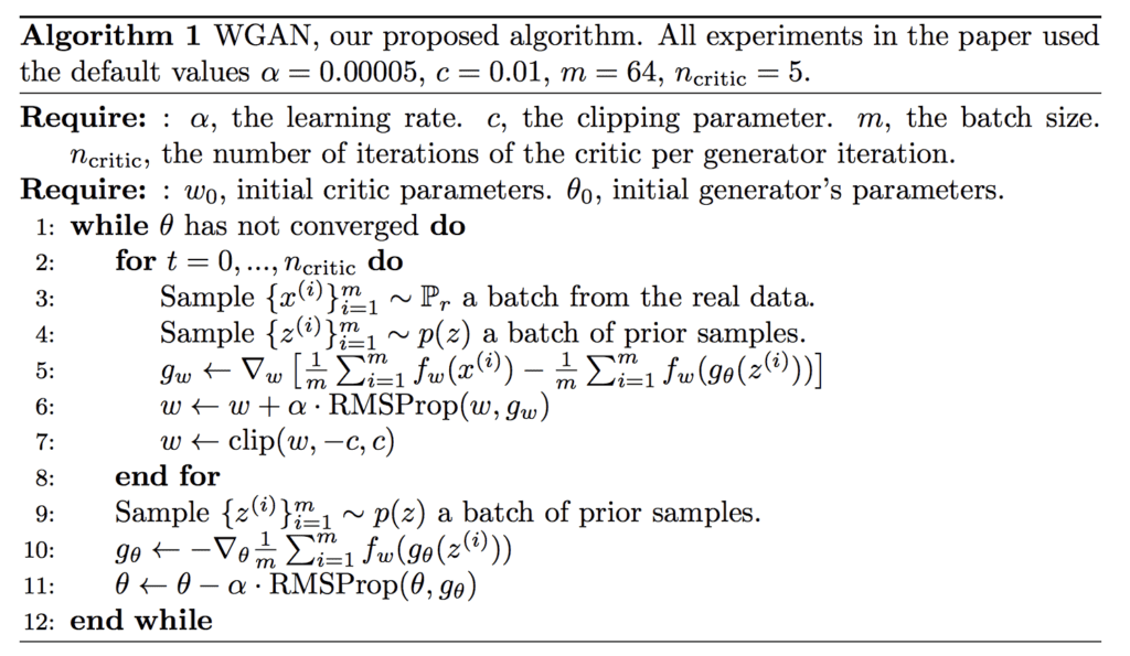
Algorithm for the Wasserstein Generative Adversarial Networks.
Taken from: Wasserstein GAN.
How to Implement Wasserstein Loss
The Wasserstein loss function seeks to increase the gap between the scores for real and generated images.
We can summarize the function as it is described in the paper as follows:
- Critic Loss = [average critic score on real images] – [average critic score on fake images]
- Generator Loss = -[average critic score on fake images]
Where the average scores are calculated across a mini-batch of samples.
This is precisely how the loss is implemented for graph-based deep learning frameworks such as PyTorch and TensorFlow.
The calculations are straightforward to interpret once we recall that stochastic gradient descent seeks to minimize loss.
In the case of the generator, a larger score from the critic will result in a smaller loss for the generator, encouraging the critic to output larger scores for fake images. For example, an average score of 10 becomes -10, an average score of 50 becomes -50, which is smaller, and so on.
In the case of the critic, a larger score for real images results in a larger resulting loss for the critic, penalizing the model. This encourages the critic to output smaller scores for real images. For example, an average score of 20 for real images and 50 for fake images results in a loss of -30; an average score of 10 for real images and 50 for fake images results in a loss of -40, which is better, and so on.
The sign of the loss does not matter in this case, as long as loss for real images is a small number and the loss for fake images is a large number. The Wasserstein loss encourages the critic to separate these numbers.
We can also reverse the situation and encourage the critic to output a large score for real images and a small score for fake images and achieve the same result. Some implementations make this change.
In the Keras deep learning library (and some others), we cannot implement the Wasserstein loss function directly as described in the paper and as implemented in PyTorch and TensorFlow. Instead, we can achieve the same effect without having the calculation of the loss for the critic dependent upon the loss calculated for real and fake images.
A good way to think about this is a negative score for real images and a positive score for fake images, although this negative/positive split of scores learned during training is not required; just larger and smaller is sufficient.
- Small Critic Score (e.g.< 0): Real – Large Critic Score (e.g. >0): Fake
We can multiply the average predicted score by -1 in the case of fake images so that larger averages become smaller averages and the gradient is in the correct direction, i.e. minimizing loss. For example, average scores on fake images of [0.5, 0.8, and 1.0] across three batches of fake images would become [-0.5, -0.8, and -1.0] when calculating weight updates.
- Loss For Fake Images = -1 * Average Critic Score
No change is needed for the case of real scores, as we want to encourage smaller average scores for real images.
- Loss For Real Images = Average Critic Score
This can be implemented consistently by assigning an expected outcome target of -1 for fake images and 1 for real images and implementing the loss function as the expected label multiplied by the average score. The -1 label will be multiplied by the average score for fake images and encourage a larger predicted average, and the +1 label will be multiplied by the average score for real images and have no effect, encouraging a smaller predicted average.
- Wasserstein Loss = Label * Average Critic Score
Or
- Wasserstein Loss(Real Images) = 1 * Average Predicted Score
- Wasserstein Loss(Fake Images) = -1 * Average Predicted Score
We can implement this in Keras by assigning the expected labels of -1 and 1 for fake and real images respectively. The inverse labels could be used to the same effect, e.g. -1 for real and +1 for fake to encourage small scores for fake images and large scores for real images. Some developers do implement the WGAN in this alternate way, which is just as correct.
The loss function can be implemented by multiplying the expected label for each sample by the predicted score (element wise), then calculating the mean.
def wasserstein_loss(y_true, y_pred):
	return mean(y_true * y_pred)
The above function is the elegant way to implement the loss function; an alternative, less-elegant implementation that might be more intuitive is as follows:
def wasserstein_loss(y_true, y_pred):
 	return mean(y_true) * mean(y_pred)
In Keras, the mean function can be implemented using the Keras backend API to ensure the mean is calculated across samples in the provided tensors; for example:
from keras import backend

# implementation of wasserstein loss
def wasserstein_loss(y_true, y_pred):
	return backend.mean(y_true * y_pred)
Now that we know how to implement the Wasserstein loss function in Keras, let’s clarify one common point of misunderstanding.
Common Point of Confusion With Expected Labels
Recall we are using the expected labels of -1 for fake images and +1 for real images.
A common point of confusion is that a perfect critic model will output -1 for every fake image and +1 for every real image.
This is incorrect.
Again, recall we are using stochastic gradient descent to find the set of weights in the critic (and generator) models that minimize the loss function.
We have established that we want the critic model to output larger scores on average for fake images and smaller scores on average for real images. We then designed a loss function to encourage this outcome.
This is the key point about loss functions used to train neural network models. They encourage a desired model behavior, and they do not have to achieve this by providing the expected outcomes. In this case, we defined our Wasserstein loss function to interpret the average score predicted by the critic model and used labels for the real and fake cases to help with this interpretation.
So what is a good loss for real and fake images under Wasserstein loss?
Wasserstein is not an absolute and comparable loss for comparing across GAN models. Instead, it is relative and depends on your model configuration and dataset. What is important is that it is consistent for a given critic model and convergence of the generator (better loss) does correlate with better generated image quality.
It could be negative scores for real images and positive scores for fake images, but this is not required. All scores could be positive or all scores could be negative.
The loss function only encourages a separation between scores for fake and real images as larger and smaller, not necessarily positive and negative.
Further Reading
This section provides more resources on the topic if you are looking to go deeper.
Papers
- Wasserstein GAN, 2017.
- WassersteinGAN, GitHub.
Articles
- Wasserstein Generative Adversarial Networks (WGANS) Project, GitHub.
- Keras-GAN: Keras implementations of Generative Adversarial Networks, GitHub.
- From GAN to WGAN, 2017.
- GAN - Wasserstein GAN & WGAN-GP, 2018.
- Improved WGAN, keras-contrib Project, GitHub.
- Wasserstein GAN, Reddit.
- Wasserstein GAN in Keras, 2017.
- Wasserstein GAN and the Kantorovich-Rubinstein Duality
- Is The WGAN Wasserstein Loss Function Correct?
Summary
In this post, you discovered how to implement Wasserstein loss for Generative Adversarial Networks.
Specifically, you learned:
- The conceptual shift in the WGAN from discriminator predicting a probability to a critic predicting a score.
- The implementation details for the WGAN as minor changes to the standard deep convolutional GAN.
- The intuition behind the Wasserstein loss function and how implement it from scratch.
Do you have any questions?
Ask your questions in the comments below and I will do my best to answer.
The post How to Implement Wasserstein Loss for Generative Adversarial Networks appeared first on Machine Learning Mastery.