
Author: Jason Brownlee
A common mistake made by beginners is to apply machine learning algorithms to a problem without establishing a performance baseline.
A performance baseline provides a minimum score above which a model is considered to have skill on the dataset. It also provides a point of relative improvement for all models evaluated on the dataset. A baseline can be established using a naive classifier, such as predicting one class label for all examples in the test dataset.
Another common mistake made by beginners is using classification accuracy as a performance metric on problems that have an imbalanced class distribution. This can result in high accuracy scores even when the majority class is predicted for all cases. Instead, an alternate performance metric must be chosen among a suite of classification measures.
The challenge is that the baseline in performance is dependent upon the choice of performance metric. As such, deep knowledge of each performance metric may be required in order to select an appropriate naive classifier to establish a performance baseline.
In this tutorial, you will discover which naive classifier to use for each imbalanced classification performance metric.
After completing this tutorial, you will know:
- The metrics to consider when evaluating machine learning models for imbalanced classification problems.
- The naive classification strategies that can be used to calculate a baseline in model performance.
- The naive classifier to use for each metric, including the rationale and a worked example demonstrating the result.
Discover SMOTE, one-class classification, cost-sensitive learning, threshold moving, and much more in my new book, with 30 step-by-step tutorials and full Python source code.
Let’s get started.

What Is the Naive Classifier for Each Imbalanced Classification Metric?
Photo by the Bureau of Land Management, some rights reserved.
Tutorial Overview
This tutorial is divided into four parts; they are:
- Metrics for Imbalanced Classification
- Naive Classification Models
- Naive Classifiers for Classification Metrics
- Naive Classifier for Accuracy
- Naive Classifier for G-Mean
- Naive Classifier for F-Measure
- Naive Classifier for ROC AUC
- Naive Classifier for Precision-Recall AUC
- Naive Classifier for Brier Score
- Summary of the Mappings
Metrics for Imbalanced Classification
There are many metrics to choose from for imbalanced classification.
Choosing a metric might be the most important step of the project, as choosing the wrong metric can result in optimizing and choosing a model that solves a problem that is different from the problem that you actually want to solve.
As such, there are perhaps 5 metrics from the tens or hundreds most commonly used that work for imbalanced classification. They are as follows:
Metrics for evaluating predicted class labels:
- Accuracy.
- G-Mean.
- F1-Measure.
- F0.5-Measure.
- F2-Measure.
Metrics for evaluating predicted probabilities:
- ROC Area Under Curve (ROC AUC).
- Precision Recall Area Under Curve (PR AUC).
- Brier Score.
For more on how to calculate each metric, see the tutorial:
Naive Classification Models
A naive classifier is a classification algorithm with no logic that provides a baseline of performance on a classification dataset.
It is important to establish a baseline in performance for a classification dataset. It provides a line in the sand by which all other algorithms can be compared. An algorithm that achieves a score below a naive classification model has no skill on the dataset, whereas an algorithm that achieves a score above that of a naive classification model has some skill on the dataset.
There are perhaps five different naive classification methods that can be used to establish a baseline of performance on a dataset.
Explained in the context of an imbalanced two-class (binary) classification problem, the naive classification methods are as follows:
- Uniformly Random Guess: Predict 0 or 1 with equal probability.
- Prior Random Guess: Predict 0 or 1 proportional to the prior probability in the dataset.
- Majority Class: Predict 0.
- Minority Class: Predict 1.
- Class Prior: Predict the prior probability for each class.
These can be implemented using the DummyClassifier class form the scikit-learn library.
This class provides the strategy argument that allows different naive classifier techniques to be used. Examples include:
- Uniformly Random Guess: Set the “strategy” argument to “uniform“.
- Prior Random Guess: Set the “strategy” argument to “stratified“.
- Majority Class: Set the “strategy” argument to “most_frequent“.
- Minority Class: Set the “strategy” argument to “constant” and set the “constant” argument to 1.
- Class Prior: Set the “strategy” argument to “prior“.
For more on naive classifiers, see the tutorial:
Want to Get Started With Imbalance Classification?
Take my free 7-day email crash course now (with sample code).
Click to sign-up and also get a free PDF Ebook version of the course.
Naive Classifiers for Classification Metrics
We have established that there are many different metrics to choose from for an imbalanced classification problem.
We have also established that it is critical to determine a baseline in performance for a new classification problem using a naive classifier.
The challenge is, each classification metric requires the careful choice of a specific naive classification strategy that achieves the appropriate “no skill” performance. This can and should be selected using knowledge of each metric and can be confirmed by careful experimentation.
In this section, we will rationalize the selection of the appropriate naive classifier for each imbalanced classification metric, then confirm the selection with an empirical result on a synthetic binary classification dataset.
The synthetic dataset has 10,000 examples, 99 percent of which belong to the majority class (negative case or class label 0) and 1 percent of which belong to the minority class (positive case or class label 1).
Each naive classifier strategy is evaluated using stratified 10-fold cross-validation with three repeats, and performance is summarized using the mean and standard deviation across these runs.
The mapping from metrics to naive classifier can be used on your next imbalanced classification project, and the empirical results confirm the rationale and help to establish the intuition for each mapping.
Let’s dive in.
Naive Classifier for Accuracy
Classification accuracy is the total number of correct predictions divided by the total number of predictions made.
The appropriate naive classifier for classification accuracy is to predict the majority class in all cases. This will maximize the true negatives and minimize the false negatives.
We can demonstrate this with a worked example comparing each naive classifier strategy on a binary classification problem. We would expect that predicting the majority class would result in a classification accuracy of approximately 99 percent on this dataset.
The complete example is listed below.
# compare naive classifiers with classification accuracy metric
from numpy import mean
from numpy import std
from sklearn.datasets import make_classification
from sklearn.model_selection import cross_val_score
from sklearn.model_selection import RepeatedStratifiedKFold
from sklearn.dummy import DummyClassifier
from matplotlib import pyplot

# evaluate a model
def evaluate_model(X, y, model):
	# define evaluation procedure
	cv = RepeatedStratifiedKFold(n_splits=10, n_repeats=3, random_state=1)
	# evaluate model
	scores = cross_val_score(model, X, y, scoring='accuracy', cv=cv, n_jobs=-1)
	return scores

# define models to test
def get_models():
	models, names = list(), list()
	# Uniformly Random Guess
	models.append(DummyClassifier(strategy='uniform'))
	names.append('Uniform')
	# Prior Random Guess
	models.append(DummyClassifier(strategy='stratified'))
	names.append('Stratified')
	# Majority Class: Predict 0
	models.append(DummyClassifier(strategy='most_frequent'))
	names.append('Majority')
	# Minority Class: Predict 1
	models.append(DummyClassifier(strategy='constant', constant=1))
	names.append('Minority')
	# Class Prior
	models.append(DummyClassifier(strategy='prior'))
	names.append('Prior')
	return models, names

# define dataset
X, y = make_classification(n_samples=10000, n_features=2, n_redundant=0,
	n_clusters_per_class=1, weights=[0.99], flip_y=0, random_state=4)
# define models
models, names = get_models()
results = list()
# evaluate each model
for i in range(len(models)):
	# evaluate the model and store results
	scores = evaluate_model(X, y, models[i])
	results.append(scores)
	# summarize and store
	print('>%s %.3f (%.3f)' % (names[i], mean(scores), std(scores)))
# plot the results
pyplot.boxplot(results, labels=names, showmeans=True)
pyplot.show()
Running the example reports the classification accuracy for each naive classifier strategy.
Your results may vary slightly given the stochastic nature of some of the methods. Try running the example a few times.
In this case, we can see that the majority strategy achieves the best classification accuracy of 99 percent, as we expected. We can also see that the prior strategy achieves the same result as it predicts mostly 0.01 (1 percent for the positive class) in all cases, which is mapped to the majority class label 0.
>Uniform 0.501 (0.015)
>Stratified 0.980 (0.003)
>Majority 0.990 (0.000)
>Minority 0.010 (0.000)
>Prior 0.990 (0.000)
Box and whisker plots for each naive classifier are also created, allowing the distribution of scores to be compared visually.
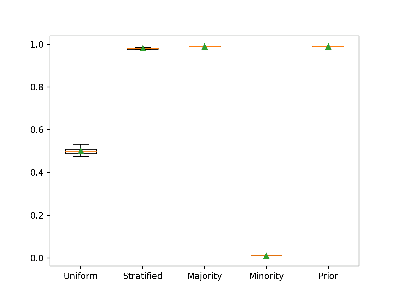
Box and Whisker Plot for Naive Classifier Strategies Evaluated Using Classification Accuracy
Naive Classifier for G-Mean
The geometric mean, or G-Mean, is the geometric mean of the sensitivity and specificity scores.
Sensitivity summarizes how well the positive class was predicted, and specificity summarizes how well the negative class was predicted.
Performing perfectly well on the majority or minority class will come at the cost of a worst-case performance on the other class, which will result in a zero G-Mean score.
Therefore, the most appropriate naive classification strategy is to predict each class with an equal probability, which will give each class an opportunity for a correct prediction.
We can demonstrate this with a worked example comparing each naive classifier strategy on a binary classification problem. We would expect that predict a uniformly random class label would result in a G-Mean of approximately 0.5 on this dataset.
The complete example is listed below.
# compare naive classifiers with g-mean metric
from numpy import mean
from numpy import std
from sklearn.datasets import make_classification
from sklearn.model_selection import cross_val_score
from sklearn.model_selection import RepeatedStratifiedKFold
from sklearn.dummy import DummyClassifier
from imblearn.metrics import geometric_mean_score
from sklearn.metrics import make_scorer
from matplotlib import pyplot

# evaluate a model
def evaluate_model(X, y, model):
	# define evaluation procedure
	cv = RepeatedStratifiedKFold(n_splits=10, n_repeats=3, random_state=1)
	# define the model evaluation the metric
	metric = make_scorer(geometric_mean_score)
	# evaluate model
	scores = cross_val_score(model, X, y, scoring=metric, cv=cv, n_jobs=-1)
	return scores

# define models to test
def get_models():
	models, names = list(), list()
	# Uniformly Random Guess
	models.append(DummyClassifier(strategy='uniform'))
	names.append('Uniform')
	# Prior Random Guess
	models.append(DummyClassifier(strategy='stratified'))
	names.append('Stratified')
	# Majority Class: Predict 0
	models.append(DummyClassifier(strategy='most_frequent'))
	names.append('Majority')
	# Minority Class: Predict 1
	models.append(DummyClassifier(strategy='constant', constant=1))
	names.append('Minority')
	# Class Prior
	models.append(DummyClassifier(strategy='prior'))
	names.append('Prior')
	return models, names

# define dataset
X, y = make_classification(n_samples=10000, n_features=2, n_redundant=0,
	n_clusters_per_class=1, weights=[0.99], flip_y=0, random_state=4)
# define models
models, names = get_models()
results = list()
# evaluate each model
for i in range(len(models)):
	# evaluate the model and store results
	scores = evaluate_model(X, y, models[i])
	results.append(scores)
	# summarize and store
	print('>%s %.3f (%.3f)' % (names[i], mean(scores), std(scores)))
# plot the results
pyplot.boxplot(results, labels=names, showmeans=True)
pyplot.show()
Running the example reports the G-mean for each naive classifier strategy.
Your results may vary slightly given the stochastic nature of some of the methods. Try running the example a few times.
In this case, we can see that, as expected, the uniformly random naive classifier resulted in a G-Mean of 0.5 and all other strategies resulted in a G-Mean score of 0.
>Uniform 0.507 (0.074)
>Stratified 0.021 (0.079)
>Majority 0.000 (0.000)
>Minority 0.000 (0.000)
>Prior 0.000 (0.000)
Box and whisker plots for each naive classifier are also created, allowing the distribution of scores to be compared visually.
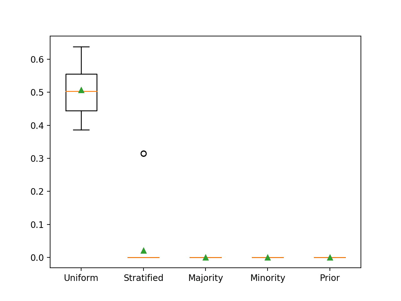
Box and Whisker Plot for Naive Classifier Strategies Evaluated Using G-Mean
Naive Classifier for F-Measure
The F-measure (also called the F1-score) is calculated as the harmonic mean between the precision and the recall.
Precision summarizes the fraction of examples assigned the positive class that belong to the positive class and recall summarizes how well the positive class was predicted out of all positive predictions that could have been made.
Making predictions that favor precision (e.g. predict the minority class) will also result in a lower bound on the recall.
Therefore, the naive strategy for the F-measure is to predict the minority class in all cases.
We can demonstrate this with a worked example comparing each naive classifier strategy on a binary classification problem.
The F-measure when predicting only the minority class for this dataset is not obvious at first. Recall will be perfect, or 1.0. The precision will be equivalent to the prior for the minority class, that is 1 percent or 0.01. Therefore, the F-measure is the harmonic mean between 1.0 and 0.01, which is about 0.02.
The complete example is listed below.
# compare naive classifiers with f1-measure
from numpy import mean
from numpy import std
from sklearn.datasets import make_classification
from sklearn.model_selection import cross_val_score
from sklearn.model_selection import RepeatedStratifiedKFold
from sklearn.dummy import DummyClassifier
from matplotlib import pyplot

# evaluate a model
def evaluate_model(X, y, model):
	# define evaluation procedure
	cv = RepeatedStratifiedKFold(n_splits=10, n_repeats=3, random_state=1)
	# evaluate model
	scores = cross_val_score(model, X, y, scoring='f1', cv=cv, n_jobs=-1)
	return scores

# define models to test
def get_models():
	models, names = list(), list()
	# Uniformly Random Guess
	models.append(DummyClassifier(strategy='uniform'))
	names.append('Uniform')
	# Prior Random Guess
	models.append(DummyClassifier(strategy='stratified'))
	names.append('Stratified')
	# Majority Class: Predict 0
	models.append(DummyClassifier(strategy='most_frequent'))
	names.append('Majority')
	# Minority Class: Predict 1
	models.append(DummyClassifier(strategy='constant', constant=1))
	names.append('Minority')
	# Class Prior
	models.append(DummyClassifier(strategy='prior'))
	names.append('Prior')
	return models, names

# define dataset
X, y = make_classification(n_samples=10000, n_features=2, n_redundant=0,
	n_clusters_per_class=1, weights=[0.99], flip_y=0, random_state=4)
# define models
models, names = get_models()
results = list()
# evaluate each model
for i in range(len(models)):
	# evaluate the model and store results
	scores = evaluate_model(X, y, models[i])
	results.append(scores)
	# summarize and store
	print('>%s %.3f (%.3f)' % (names[i], mean(scores), std(scores)))
# plot the results
pyplot.boxplot(results, labels=names, showmeans=True)
pyplot.show()
Running the example reports the ROC AUC for each naive classifier strategy.
Your results may vary slightly given the stochastic nature of some of the methods. Try running the example a few times.
You may get a warning when evaluating the naive classifier that only predicts the minority class, as there are no positive cases predicted. You will see a warning as follows:
UndefinedMetricWarning: F-score is ill-defined and being set to 0.0 due to no predicted samples.
In this case, we can see that predicting the minority class results in the expected F-measure of about 0.02. We can also see that we approximate this score when using the uniform and stratified strategies.
>Uniform 0.020 (0.007)
>Stratified 0.020 (0.040)
>Majority 0.000 (0.000)
>Minority 0.020 (0.000)
>Prior 0.000 (0.000)
Box and whisker plots for each naive classifier are also created, allowing the distribution of scores to be compared visually.
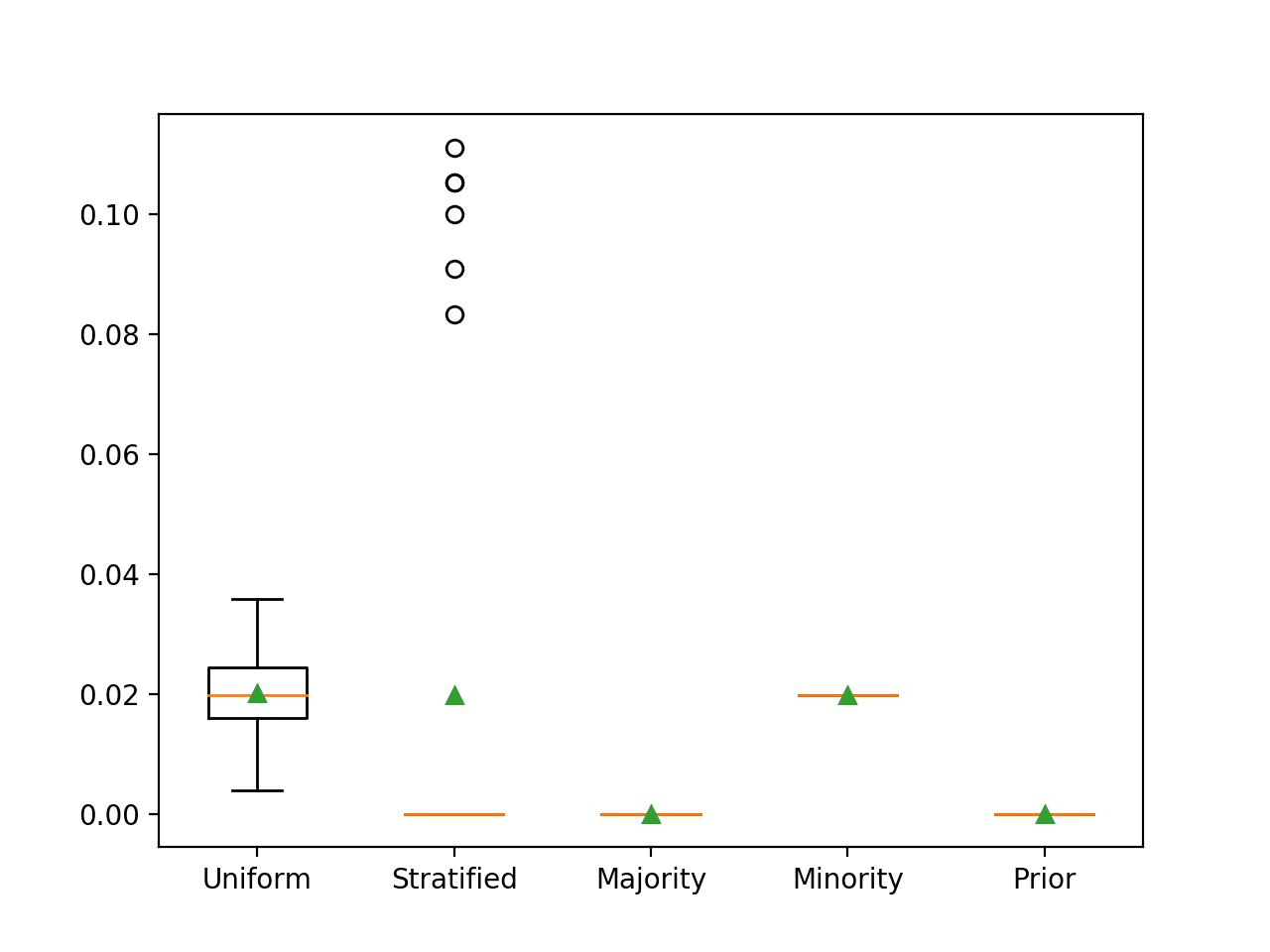
Box and Whisker Plot for Naive Classifier Strategies Evaluated Using F-Measure
This same naive classifier strategy of predicting the minority class is also appropriate when using the F0.5 and F2 measures.
Naive Classifier for ROC AUC
The ROC Curve is a plot of the false positive rate versus the true positive rate for a range of different probability thresholds.
The ROC area under curve is an approximation of the integral or area under the ROC curve and summarizes how well an algorithm performs across the range of probability thresholds.
A no-skill model has a ROC AUC of 0.5 and can be achieved by predicting class labels randomly but in proportion to their base rate (e.g. no discrimination power). This would be the stratified method.
Predicting a constant value, like the majority class or minority class will result in an invalid ROC Curve (e.g. a point) and in turn an invalid ROC AUC score. Scores for models that predict a constant value should be ignored.
The complete example is listed below.
# compare naive classifiers with roc auc
from numpy import mean
from numpy import std
from sklearn.datasets import make_classification
from sklearn.model_selection import cross_val_score
from sklearn.model_selection import RepeatedStratifiedKFold
from sklearn.dummy import DummyClassifier
from matplotlib import pyplot

# evaluate a model
def evaluate_model(X, y, model):
	# define evaluation procedure
	cv = RepeatedStratifiedKFold(n_splits=10, n_repeats=3, random_state=1)
	# evaluate model
	scores = cross_val_score(model, X, y, scoring='roc_auc', cv=cv, n_jobs=-1)
	return scores

# define models to test
def get_models():
	models, names = list(), list()
	# Uniformly Random Guess
	models.append(DummyClassifier(strategy='uniform'))
	names.append('Uniform')
	# Prior Random Guess
	models.append(DummyClassifier(strategy='stratified'))
	names.append('Stratified')
	# Majority Class: Predict 0
	models.append(DummyClassifier(strategy='most_frequent'))
	names.append('Majority')
	# Minority Class: Predict 1
	models.append(DummyClassifier(strategy='constant', constant=1))
	names.append('Minority')
	# Class Prior
	models.append(DummyClassifier(strategy='prior'))
	names.append('Prior')
	return models, names

# define dataset
X, y = make_classification(n_samples=10000, n_features=2, n_redundant=0,
	n_clusters_per_class=1, weights=[0.99], flip_y=0, random_state=4)
# define models
models, names = get_models()
results = list()
# evaluate each model
for i in range(len(models)):
	# evaluate the model and store results
	scores = evaluate_model(X, y, models[i])
	results.append(scores)
	# summarize and store
	print('>%s %.3f (%.3f)' % (names[i], mean(scores), std(scores)))
# plot the results
pyplot.boxplot(results, labels=names, showmeans=True)
pyplot.show()
Running the example reports the ROC AUC for each naive classifier strategy.
Your results may vary slightly given the stochastic nature of some of the methods. Try running the example a few times.
In this case, we can see that as expected, predicting a stratified random label results in the worst-case ROC AUC of 0.5.
>Uniform 0.500 (0.000)
>Stratified 0.506 (0.020)
>Majority 0.500 (0.000)
>Minority 0.500 (0.000)
>Prior 0.500 (0.000)
Box and whisker plots for each naive classifier are also created, allowing the distribution of scores to be compared visually.
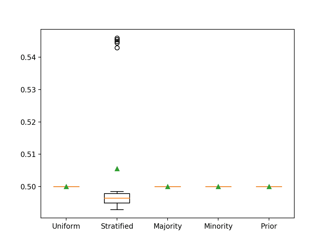
Box and Whisker Plot for Naive Classifier Strategies Evaluated Using ROC AUC
Naive Classifier for Precision-Recall AUC
The Precision-Recall Curve (or PR Curve) is a plot of the recall versus the precision for a range of different probability thresholds.
The Precision-Recall area under curve is an approximation of the integral or area under the Precision-Recall curve and summarizes how well an algorithm performs across the range of probability thresholds.
A no-skill model has a PR AUC that matches the base rate of the positive class, e.g. 0.01. This can be achieved by predicting class labels randomly but in proportion to their base rate (e.g. no discrimination power). This would be the stratified method.
Predicting a constant value, like the majority class or minority class will result in an invalid PR Curve (e.g. a point) and in turn an invalid PR AUC score. Scores for models that predict a constant value should be ignored.
The complete example is listed below.
# compare naive classifiers with precision-recall auc metric
from numpy import mean
from numpy import std
from sklearn.datasets import make_classification
from sklearn.model_selection import cross_val_score
from sklearn.model_selection import RepeatedStratifiedKFold
from sklearn.dummy import DummyClassifier
from sklearn.metrics import precision_recall_curve
from sklearn.metrics import auc
from sklearn.metrics import make_scorer
from matplotlib import pyplot

# calculate precision-recall area under curve
def pr_auc(y_true, probas_pred):
	# calculate precision-recall curve
	p, r, _ = precision_recall_curve(y_true, probas_pred)
	# calculate area under curve
	return auc(r, p)

# evaluate a model
def evaluate_model(X, y, model):
	# define evaluation procedure
	cv = RepeatedStratifiedKFold(n_splits=10, n_repeats=3, random_state=1)
	# define the model evaluation the metric
	metric = make_scorer(pr_auc, needs_proba=True)
	# evaluate model
	scores = cross_val_score(model, X, y, scoring=metric, cv=cv, n_jobs=-1)
	return scores

# define models to test
def get_models():
	models, names = list(), list()
	# Uniformly Random Guess
	models.append(DummyClassifier(strategy='uniform'))
	names.append('Uniform')
	# Prior Random Guess
	models.append(DummyClassifier(strategy='stratified'))
	names.append('Stratified')
	# Majority Class: Predict 0
	models.append(DummyClassifier(strategy='most_frequent'))
	names.append('Majority')
	# Minority Class: Predict 1
	models.append(DummyClassifier(strategy='constant', constant=1))
	names.append('Minority')
	# Class Prior
	models.append(DummyClassifier(strategy='prior'))
	names.append('Prior')
	return models, names

# define dataset
X, y = make_classification(n_samples=10000, n_features=2, n_redundant=0,
	n_clusters_per_class=1, weights=[0.99], flip_y=0, random_state=4)
# define models
models, names = get_models()
results = list()
# evaluate each model
for i in range(len(models)):
	# evaluate the model and store results
	scores = evaluate_model(X, y, models[i])
	results.append(scores)
	# summarize and store
	print('>%s %.3f (%.3f)' % (names[i], mean(scores), std(scores)))
# plot the results
pyplot.boxplot(results, labels=names, showmeans=True)
pyplot.show()
Running the example reports the PR AUC score for each naive classifier strategy.
Your results may vary slightly given the stochastic nature of some of the methods. Try running the example a few times.
In this case, we can see that as expected, predicting a stratified random class label results in the worst-case PR AUC of close to 0.01.
>Uniform 0.505 (0.000)
>Stratified 0.015 (0.037)
>Majority 0.505 (0.000)
>Minority 0.505 (0.000)
>Prior 0.505 (0.000)
Box and whisker plots for each naive classifier are also created, allowing the distribution of scores to be compared visually.
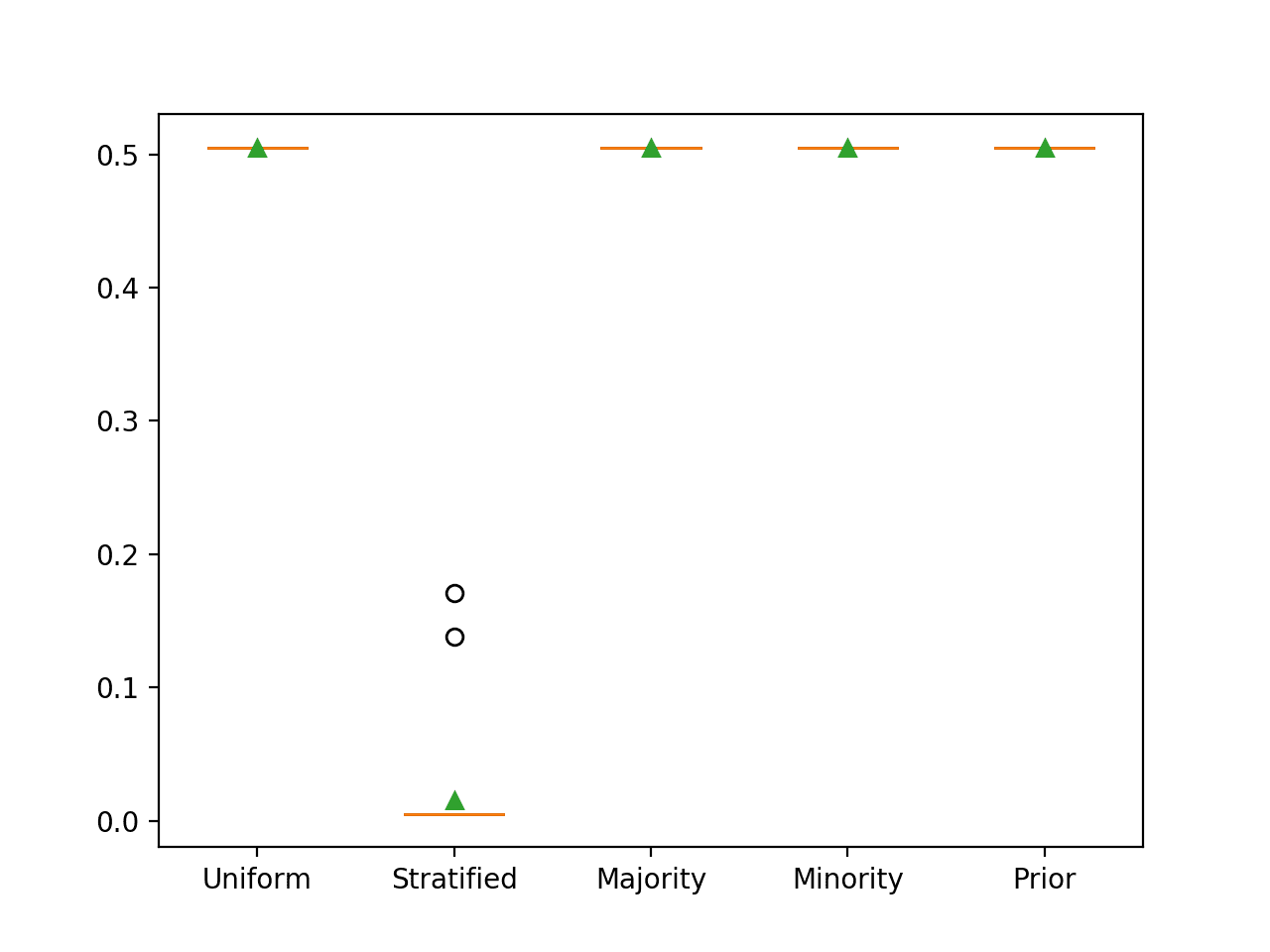
Box and Whisker Plot for Naive Classifier Strategies Evaluated Using Precision-Recall AUC
Naive Classifier for Brier Score
Brier score calculates the mean squared error between the expected probabilities and the predicted probabilities.
The appropriate naive classifier for Brier score is to predict the class priors for each example in the test set. For a binary classification problem that involves predicting a Binomial distribution, this would be the prior for class 0 and the prior for class 1.
We can demonstrate this with a worked example comparing each naive classifier strategy on a binary classification problem.
The model would predict the probabilities [0.99, 0.01] in all cases. We would expect that this will result in mean squared error close to the prior for the minority class, e.g. 0.01 on this dataset. This is because the Binomial probability for most examples is 0.0 with only 1 percent having 1.0 which results in a maximum error for 1 percent of cases, or a Brier score of 0.01.
The complete example is listed below.
# compare naive classifiers with brier score metric
from numpy import mean
from numpy import std
from sklearn.datasets import make_classification
from sklearn.model_selection import cross_val_score
from sklearn.model_selection import RepeatedStratifiedKFold
from sklearn.dummy import DummyClassifier
from matplotlib import pyplot

# evaluate a model
def evaluate_model(X, y, model):
	# define evaluation procedure
	cv = RepeatedStratifiedKFold(n_splits=10, n_repeats=3, random_state=1)
	# evaluate model
	scores = cross_val_score(model, X, y, scoring='brier_score_loss', cv=cv, n_jobs=-1)
	return scores

# define models to test
def get_models():
	models, names = list(), list()
	# Uniformly Random Guess
	models.append(DummyClassifier(strategy='uniform'))
	names.append('Uniform')
	# Prior Random Guess
	models.append(DummyClassifier(strategy='stratified'))
	names.append('Stratified')
	# Majority Class: Predict 0
	models.append(DummyClassifier(strategy='most_frequent'))
	names.append('Majority')
	# Minority Class: Predict 1
	models.append(DummyClassifier(strategy='constant', constant=1))
	names.append('Minority')
	# Class Prior
	models.append(DummyClassifier(strategy='prior'))
	names.append('Prior')
	return models, names

# define dataset
X, y = make_classification(n_samples=10000, n_features=2, n_redundant=0,
	n_clusters_per_class=1, weights=[0.99], flip_y=0, random_state=4)
# define models
models, names = get_models()
results = list()
# evaluate each model
for i in range(len(models)):
	# evaluate the model and store results
	scores = evaluate_model(X, y, models[i])
	results.append(scores)
	# summarize and store
	print('>%s %.3f (%.3f)' % (names[i], mean(scores), std(scores)))
# plot the results
pyplot.boxplot(results, labels=names, showmeans=True)
pyplot.show()
Running the example reports the Brier score for each naive classifier strategy.
Your results may vary slightly given the stochastic nature of some of the methods. Try running the example a few times.
Brier score is minimized, with 0.0 representing the lowest possible score.
As such, the scikit-learn inverts the score by making it negative, hence the negative mean Brier scores for each naive classifier. The sign can, therefore, be ignored.
As expected, we can see that predicting the prior probability results in the best score. We can also see that predicting the majority class also results in the same best Brier score.
>Uniform -0.250 (0.000)
>Stratified -0.020 (0.003)
>Majority -0.010 (0.000)
>Minority -0.990 (0.000)
>Prior -0.010 (0.000)
Box and whisker plots for each naive classifier are also created, allowing the distribution of scores to be compared visually.
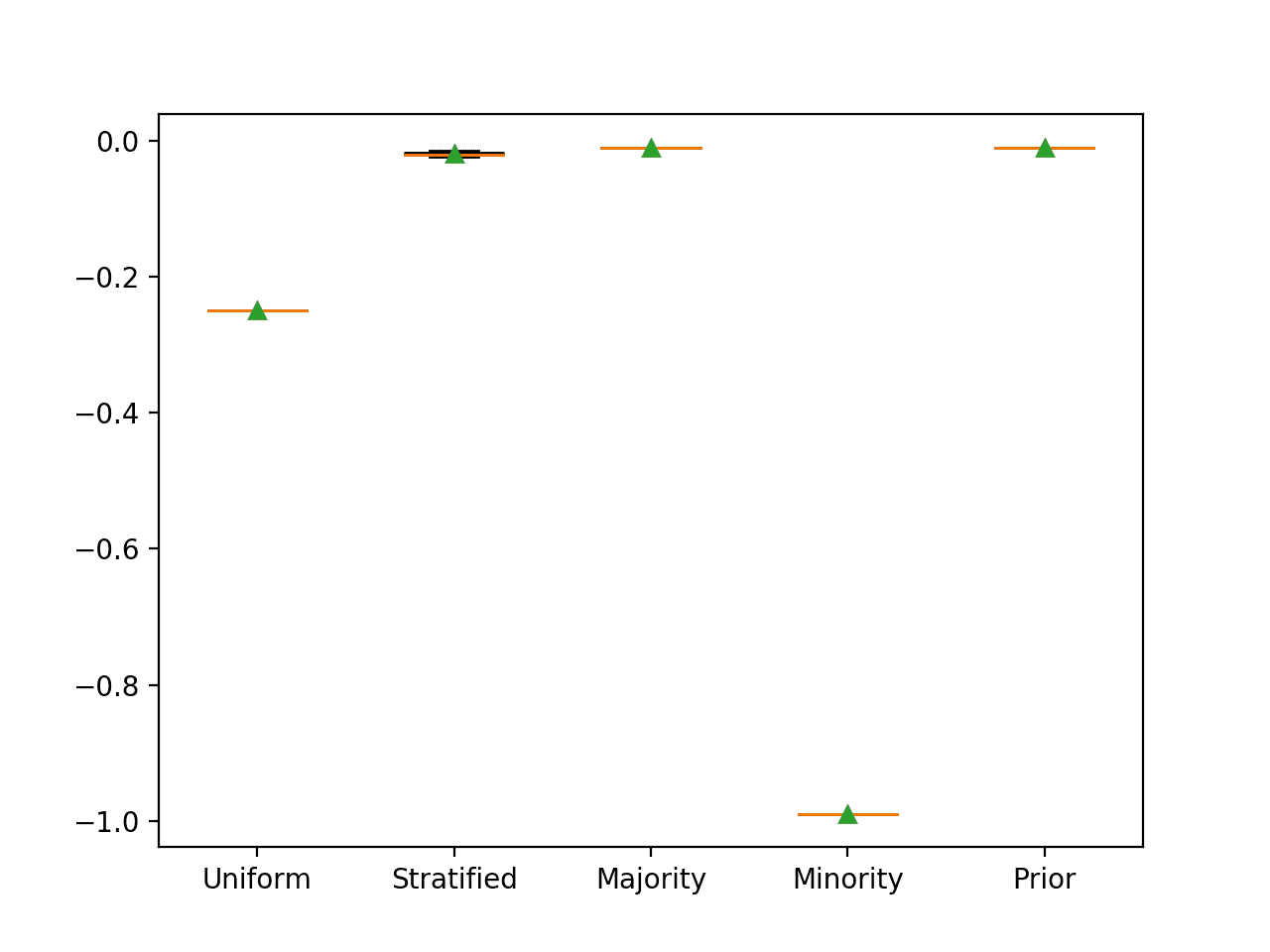
Box and Whisker Plot for Naive Classifier Strategies Evaluated Using Brier Score
Summary of the Mappings
We can summarize the mapping of imbalanced classification metrics to naive classification methods.
This provides a look-up table that you can consult on your next imbalanced classification project.
- Accuracy: Predict the majority class (class 0).
- G-Mean: Predict a uniformly random class.
- F1-Measure: Predict the minority class (class 1).
- F0.5-Measure: Predict the minority class (class 1).
- F2-Measure: Predict the minority class (class 1).
- ROC AUC: Predict a stratified random class.
- PR ROC: Predict a stratified random class.
- Brier Score: Predict majority class prior.
Further Reading
This section provides more resources on the topic if you are looking to go deeper.
Tutorials
- Tour of Evaluation Metrics for Imbalanced Classification
- How to Develop and Evaluate Naive Classifier Strategies Using Probability
APIs
Summary
In this tutorial, you discovered which naive classifier to use for each imbalanced classification performance metric.
Specifically, you learned:
- The metrics to consider when evaluating machine learning models for imbalanced classification problems.
- The naive classification strategies that can be used to calculate a baseline in model performance.
- The naive classifier to use for each metric, including the rationale and a worked example demonstrating the result.
Do you have any questions?
Ask your questions in the comments below and I will do my best to answer.
The post What Is the Naive Classifier for Each Imbalanced Classification Metric? appeared first on Machine Learning Mastery.