Author: Kevin Mekulu
Summary
- Monte Carlo simulation is one of the most important algorithms in quantitative finance
- Monte Carlo simulation can be utilized as an alternative tool to price options ( the most popular option pricing model is based on the Black-Scholes-Merton formula)
How Does Monte Carlo Simulation Work?
Before demonstrating the implementation of the Monte Carlo algorithm, it’s important to fully comprehend the science behind it. Simply put, Monte Carlo simulation generates a series of random variables that have similar properties to the risk factors which the simulation is trying to simulate.
The simulation produces a large number of possible outcomes along with their probabilities. In summary, it’s used to simulate realistic scenarios (stock prices, option prices, probabilities…).
Note: Monte Carlo simulations can get computationally expensive and slow depending on the number of generated scenarios.
Next, I will demonstrate how we can leverage Monte Carlo simulation to price a European call option and implement its algorithm in Python.
Pricing a European Call Option Using Monte Carlo Simulation
Let’s start by looking at the famous Black-Scholes-Merton formula (1973):
Equation 3–1: Black-Scholes-Merton Stochastic Differential Equation (SDE)
S(t) = Stock price at time t
r = Risk free rate
σ = Volatility
Z(t) = Brownian motion
Our goal is to solve the equation above to obtain an explicit formula for S(t).
We utilized Euler Discretization Scheme to solve the stochastic equation above. The solution is given by the expression:

Equation 3–2: Euler Discretization of SDE
Let’s apply the logarithm function to equation 3–2 above which will allow a faster implementation in Python (the vectorization process using the numpy package in Python would easily ingest the log version of the solution above).

Equation 3–3: Euler Discretization of SDE (log version)
Monte Carlo Implementation in Python
We will utilize the numpy package and its vectorization properties to make the program more compact, easier to read, maintain and faster to execute. The source code below is available here.
#
# Monte Carlo valuation of European call options with NumPy (log version)
# Monte_Carlo.py
#
import math
from numpy import *
from time import time
# star import for shorter code
random.seed(20000)
t0 = time()
# Parameters
S0 = 100.; K = 105.; T = 1.0; r = 0.05; sigma = 0.2
M = 50; dt = T / M; I = 250000
# Simulating I paths with M time steps
S = S0 * exp(cumsum((r – 0.5 * sigma ** 2) * dt
+ sigma * math.sqrt(dt)
* random.standard_normal((M + 1, I)), axis=0))
# sum instead of cumsum would also do
# if only the final values are of interest
S[0] = S0
# Calculating the Monte Carlo estimator
C0 = math.exp(-r * T) * sum(maximum(S[-1] – K, 0)) / I
# Results output
tnp2 = time() – t0
print(‘The European Option Value is: ‘, C0) # The European Option Value is: 8.165807966259603
print(‘The Execution Time is: ‘,tnp2) # The Execution Time is: 0.9024488925933838
Graphical Visualization
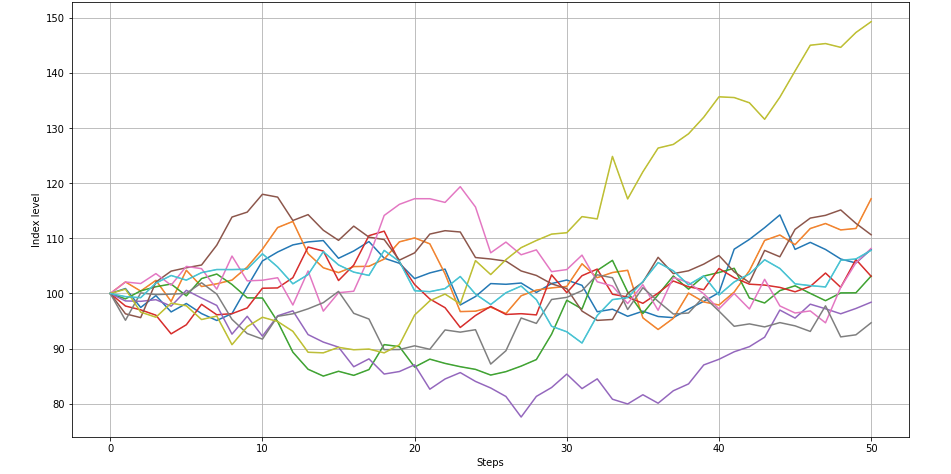
The graph below displays a plot of the first 10 simulated paths. Those simulated paths represent different outcomes for the price of the underlying asset (index level).
import matplotlib.pyplot as plt
plt.plot(S[:, :10])

plt.grid(True)

plt.xlabel('Steps')

plt.ylabel('Index level')

plt.show()

Figure 3–1: Simulated index levels by time steps
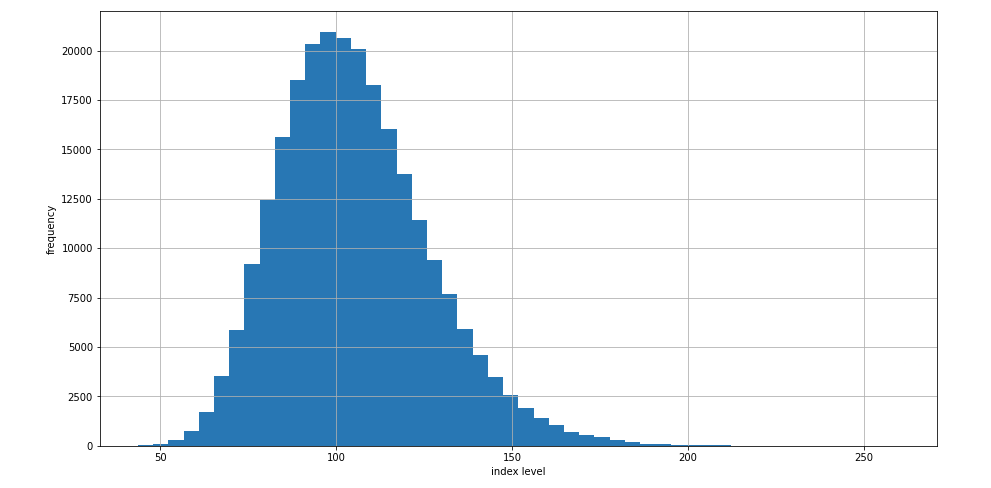
Next, let’s investigate the frequency of the simulated index levels at the end of the simulation period.
plt.rcParams["figure.figsize"] = (15,8)
plt.hist(S[-1], bins=50)

plt.grid(True)

plt.xlabel('index level')

plt.ylabel('frequency')

Figure 3–2: Histogram of all simulated end-of-period index values
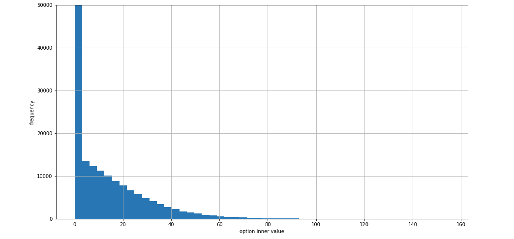
Next, let’s look at the histogram of all simulated end-of-period option values.
import numpy as np
plt.rcParams["figure.figsize"] = (15,8)

plt.hist(np.maximum(S[-1] - K, 0), bins=50)

plt.grid(True)

plt.xlabel('option inner value')

plt.ylabel('frequency')

plt.ylim(0, 50000)

Figure 3–3: Histogram of all simulated option values
We notice something very interesting in the latter plot. The European call option expires worthless the majority of the time. This might be useful information for an astute options trader! But that’s a discussion for another day.
References
Hilpisch, Y. (2015). Python for Finance: Analyze Big Financial Data
Originally posted here
