
Author: Jason Brownlee
Gradient descent is an optimization algorithm that follows the negative gradient of an objective function in order to locate the minimum of the function.
A limitation of gradient descent is that a single step size (learning rate) is used for all input variables. Extensions to gradient descent, like the Adaptive Movement Estimation (Adam) algorithm, use a separate step size for each input variable but may result in a step size that rapidly decreases to very small values.
AdaMax is an extension to the Adam version of gradient descent that generalizes the approach to the infinite norm (max) and may result in a more effective optimization on some problems.
In this tutorial, you will discover how to develop gradient descent optimization with AdaMax from scratch.
After completing this tutorial, you will know:
- Gradient descent is an optimization algorithm that uses the gradient of the objective function to navigate the search space.
- AdaMax is an extension of the Adam version of gradient descent designed to accelerate the optimization process.
- How to implement the AdaMax optimization algorithm from scratch and apply it to an objective function and evaluate the results.
Let’s get started.

Gradient Descent Optimization With AdaMax From Scratch
Photo by Don Graham, some rights reserved.
Tutorial Overview
This tutorial is divided into three parts; they are:
- Gradient Descent
- AdaMax Optimization Algorithm
- Gradient Descent With AdaMax
- Two-Dimensional Test Problem
- Gradient Descent Optimization With AdaMax
- Visualization of AdaMax Optimization
Gradient Descent
Gradient descent is an optimization algorithm.
It is technically referred to as a first-order optimization algorithm as it explicitly makes use of the first-order derivative of the target objective function.
First-order methods rely on gradient information to help direct the search for a minimum …
— Page 69, Algorithms for Optimization, 2019.
The first-order derivative, or simply the “derivative,” is the rate of change or slope of the target function at a specific point, e.g. for a specific input.
If the target function takes multiple input variables, it is referred to as a multivariate function and the input variables can be thought of as a vector. In turn, the derivative of a multivariate target function may also be taken as a vector and is referred to generally as the gradient.
- Gradient: First-order derivative for a multivariate objective function.
The derivative or the gradient points in the direction of the steepest ascent of the target function for a specific input.
Gradient descent refers to a minimization optimization algorithm that follows the negative of the gradient downhill of the target function to locate the minimum of the function.
The gradient descent algorithm requires a target function that is being optimized and the derivative function for the objective function. The target function f() returns a score for a given set of inputs, and the derivative function f'() gives the derivative of the target function for a given set of inputs.
The gradient descent algorithm requires a starting point (x) in the problem, such as a randomly selected point in the input space.
The derivative is then calculated and a step is taken in the input space that is expected to result in a downhill movement in the target function, assuming we are minimizing the target function.
A downhill movement is made by first calculating how far to move in the input space, calculated as the step size (called alpha or the learning rate) multiplied by the gradient. This is then subtracted from the current point, ensuring we move against the gradient, or down the target function.
- x(t) = x(t-1) – step_size * f'(x(t))
The steeper the objective function at a given point, the larger the magnitude of the gradient, and in turn, the larger the step taken in the search space. The size of the step taken is scaled using a step size hyperparameter.
- Step Size: Hyperparameter that controls how far to move in the search space against the gradient each iteration of the algorithm.
If the step size is too small, the movement in the search space will be small and the search will take a long time. If the step size is too large, the search may bounce around the search space and skip over the optima.
Now that we are familiar with the gradient descent optimization algorithm, let’s take a look at the AdaMax algorithm.
AdaMax Optimization Algorithm
AdaMax algorithm is an extension to the Adaptive Movement Estimation (Adam) Optimization algorithm. More broadly, is an extension to the Gradient Descent Optimization algorithm.
The algorithm was described in the 2014 paper by Diederik Kingma and Jimmy Lei Ba titled “Adam: A Method for Stochastic Optimization.”
Adam can be understood as updating weights inversely proportional to the scaled L2 norm (squared) of past gradients. AdaMax extends this to the so-called infinite norm (max) of past gradients.
In Adam, the update rule for individual weights is to scale their gradients inversely proportional to a (scaled) L^2 norm of their individual current and past gradients
— Adam: A Method for Stochastic Optimization, 2014.
Generally, AdaMax automatically adapts a separate step size (learning rate) for each parameter in the optimization problem.
Let’s step through each element of the algorithm.
First, we must maintain a moment vector and exponentially weighted infinity norm for each parameter being optimized as part of the search, referred to as m and u respectively.
They are initialized to 0.0 at the start of the search.
- m = 0
- u = 0
The algorithm is executed iteratively over time t starting at t=1, and each iteration involves calculating a new set of parameter values x, e.g. going from x(t-1) to x(t).
It is perhaps easy to understand the algorithm if we focus on updating one parameter, which generalizes to updating all parameters via vector operations.
First, the gradient (partial derivatives) are calculated for the current time step.
- g(t) = f'(x(t-1))
Next, the moment vector is updated using the gradient and a hyperparameter beta1.
- m(t) = beta1 * m(t-1) + (1 – beta1) * g(t)
The exponentially weighted infinity norm is updated using the beta2 hyperparameter.
- u(t) = max(beta2 * u(t-1), abs(g(t)))
Where max() selects the maximum of the parameters and abs() calculates the absolute value.
We can then update the parameter value. This can be broken down into three pieces; the first calculates the step size parameter, the second the gradient, and the third uses the step size and gradient to calculate the new parameter value.
Let’s start with calculating the step size for the parameter using an initial step size hyperparameter called alpha and a version of beta1 that is decaying over time with a specific value for this time step beta1(t):
- step_size(t) = alpha / (1 – beta1(t))
The gradient used for updating the parameter is calculated as follows:
- delta(t) = m(t) / u(t)
Finally, we can calculate the value for the parameter for this iteration.
- x(t) = x(t-1) – step_size(t) * delta(t)
Or the complete update equation can be stated as:
- x(t) = x(t-1) – (alpha / (1 – beta1(t))) * m(t) / u(t)
To review, there are three hyperparameters for the algorithm; they are:
- alpha: Initial step size (learning rate), a typical value is 0.002.
- beta1: Decay factor for first momentum, a typical value is 0.9.
- beta2: Decay factor for infinity norm, a typical value is 0.999.
The decay schedule for beta1(t) suggested in the paper is calculated using the initial beta1 value raised to the power t, although other decay schedules could be used such as holding the value constant or decaying more aggressively.
- beta1(t) = beta1^t
And that’s it.
For the full derivation of the AdaMax algorithm in the context of the Adam algorithm, I recommend reading the paper:
Next, let’s look at how we might implement the algorithm from scratch in Python.
Gradient Descent With AdaMax
In this section, we will explore how to implement the gradient descent optimization algorithm with AdaMax Momentum.
Two-Dimensional Test Problem
First, let’s define an optimization function.
We will use a simple two-dimensional function that squares the input of each dimension and define the range of valid inputs from -1.0 to 1.0.
The objective() function below implements this.
# objective function
def objective(x, y):
	return x**2.0 + y**2.0
We can create a three-dimensional plot of the dataset to get a feeling for the curvature of the response surface.
The complete example of plotting the objective function is listed below.
# 3d plot of the test function
from numpy import arange
from numpy import meshgrid
from matplotlib import pyplot

# objective function
def objective(x, y):
	return x**2.0 + y**2.0

# define range for input
r_min, r_max = -1.0, 1.0
# sample input range uniformly at 0.1 increments
xaxis = arange(r_min, r_max, 0.1)
yaxis = arange(r_min, r_max, 0.1)
# create a mesh from the axis
x, y = meshgrid(xaxis, yaxis)
# compute targets
results = objective(x, y)
# create a surface plot with the jet color scheme
figure = pyplot.figure()
axis = figure.gca(projection='3d')
axis.plot_surface(x, y, results, cmap='jet')
# show the plot
pyplot.show()
Running the example creates a three-dimensional surface plot of the objective function.
We can see the familiar bowl shape with the global minima at f(0, 0) = 0.
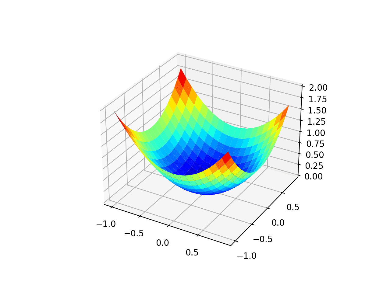
Three-Dimensional Plot of the Test Objective Function
We can also create a two-dimensional plot of the function. This will be helpful later when we want to plot the progress of the search.
The example below creates a contour plot of the objective function.
# contour plot of the test function
from numpy import asarray
from numpy import arange
from numpy import meshgrid
from matplotlib import pyplot

# objective function
def objective(x, y):
	return x**2.0 + y**2.0

# define range for input
bounds = asarray([[-1.0, 1.0], [-1.0, 1.0]])
# sample input range uniformly at 0.1 increments
xaxis = arange(bounds[0,0], bounds[0,1], 0.1)
yaxis = arange(bounds[1,0], bounds[1,1], 0.1)
# create a mesh from the axis
x, y = meshgrid(xaxis, yaxis)
# compute targets
results = objective(x, y)
# create a filled contour plot with 50 levels and jet color scheme
pyplot.contourf(x, y, results, levels=50, cmap='jet')
# show the plot
pyplot.show()
Running the example creates a two-dimensional contour plot of the objective function.
We can see the bowl shape compressed to contours shown with a color gradient. We will use this plot to plot the specific points explored during the progress of the search.
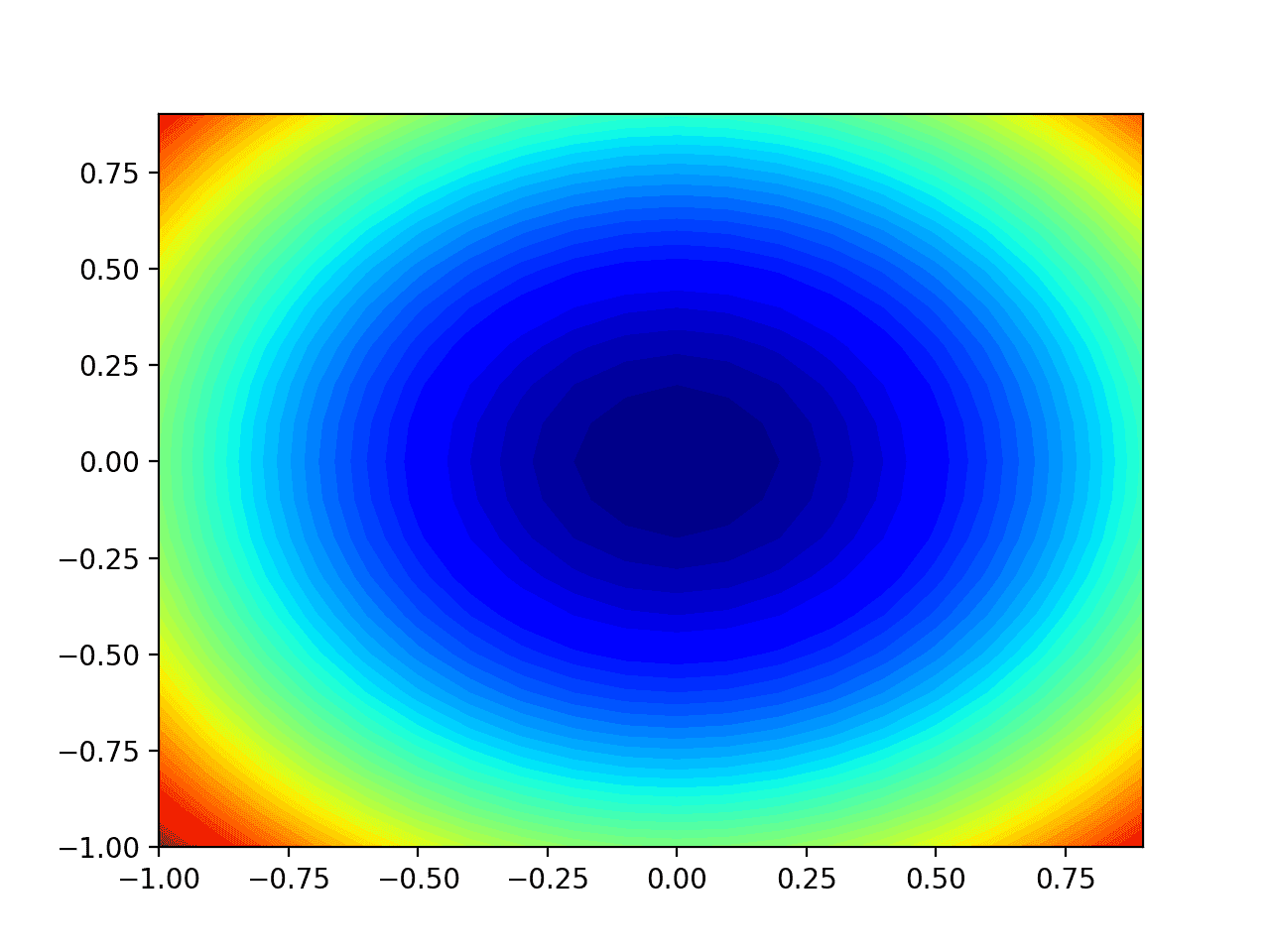
Two-Dimensional Contour Plot of the Test Objective Function
Now that we have a test objective function, let’s look at how we might implement the AdaMax optimization algorithm.
Gradient Descent Optimization With AdaMax
We can apply the gradient descent with AdaMax to the test problem.
First, we need a function that calculates the derivative for this function.
The derivative of x^2 is x * 2 in each dimension.
- f(x) = x^2
- f'(x) = x * 2
The derivative() function implements this below.
# derivative of objective function
def derivative(x, y):
	return asarray([x * 2.0, y * 2.0])
Next, we can implement gradient descent optimization with AdaMax.
First, we can select a random point in the bounds of the problem as a starting point for the search.
This assumes we have an array that defines the bounds of the search with one row for each dimension and the first column defines the minimum and the second column defines the maximum of the dimension.
...
# generate an initial point
x = bounds[:, 0] + rand(len(bounds)) * (bounds[:, 1] - bounds[:, 0])
Next, we need to initialize the moment vector and exponentially weighted infinity norm.
...
# initialize moment vector and weighted infinity norm
m = [0.0 for _ in range(bounds.shape[0])]
u = [0.0 for _ in range(bounds.shape[0])]
We then run a fixed number of iterations of the algorithm defined by the “n_iter” hyperparameter.
...
# run iterations of gradient descent
for t in range(n_iter):
	...
The first step is to calculate the derivative for the current set of parameters.
...
# calculate gradient g(t)
g = derivative(x[0], x[1])
Next, we need to perform the AdaMax update calculations. We will perform these calculations one variable at a time using an imperative programming style for readability.
In practice, I recommend using NumPy vector operations for efficiency.
...
# build a solution one variable at a time
for i in range(x.shape[0]):
	...
First, we need to calculate the moment vector.
...
# m(t) = beta1 * m(t-1) + (1 - beta1) * g(t)
m[i] = beta1 * m[i] + (1.0 - beta1) * g[i]
Next, we need to calculate the exponentially weighted infinity norm.
...
# u(t) = max(beta2 * u(t-1), abs(g(t)))
u[i] = max(beta2 * u[i], abs(g[i]))
Then the step size used in the update.
...
# step_size(t) = alpha / (1 - beta1(t))
step_size = alpha / (1.0 - beta1**(t+1))
And the change in variable.
...
# delta(t) = m(t) / u(t)
delta = m[i] / u[i]
Finally, we can calculate the new value for the variable.
...
# x(t) = x(t-1) - step_size(t) * delta(t)
x[i] = x[i] - step_size * delta
This is then repeated for each parameter that is being optimized.
At the end of the iteration, we can evaluate the new parameter values and report the performance of the search.
...
# evaluate candidate point
score = objective(x[0], x[1])
# report progress
print('>%d f(%s) = %.5f' % (t, x, score))
We can tie all of this together into a function named adamax() that takes the names of the objective and derivative functions as well as the algorithm hyperparameters and returns the best solution found at the end of the search and its evaluation.
# gradient descent algorithm with adamax
def adamax(objective, derivative, bounds, n_iter, alpha, beta1, beta2):
	# generate an initial point
	x = bounds[:, 0] + rand(len(bounds)) * (bounds[:, 1] - bounds[:, 0])
	# initialize moment vector and weighted infinity norm
	m = [0.0 for _ in range(bounds.shape[0])]
	u = [0.0 for _ in range(bounds.shape[0])]
	# run iterations of gradient descent
	for t in range(n_iter):
		# calculate gradient g(t)
		g = derivative(x[0], x[1])
		# build a solution one variable at a time
		for i in range(x.shape[0]):
			# m(t) = beta1 * m(t-1) + (1 - beta1) * g(t)
			m[i] = beta1 * m[i] + (1.0 - beta1) * g[i]
			# u(t) = max(beta2 * u(t-1), abs(g(t)))
			u[i] = max(beta2 * u[i], abs(g[i]))
			# step_size(t) = alpha / (1 - beta1(t))
			step_size = alpha / (1.0 - beta1**(t+1))
			# delta(t) = m(t) / u(t)
			delta = m[i] / u[i]
			# x(t) = x(t-1) - step_size(t) * delta(t)
			x[i] = x[i] - step_size * delta
		# evaluate candidate point
		score = objective(x[0], x[1])
		# report progress
		print('>%d f(%s) = %.5f' % (t, x, score))
	return [x, score]
We can then define the bounds of the function and the hyperparameters and call the function to perform the optimization.
In this case, we will run the algorithm for 60 iterations with an initial learning rate of 0.02, beta of 0.8, and a beta2 of 0.99, found after a little trial and error.
...
# seed the pseudo random number generator
seed(1)
# define range for input
bounds = asarray([[-1.0, 1.0], [-1.0, 1.0]])
# define the total iterations
n_iter = 60
# steps size
alpha = 0.02
# factor for average gradient
beta1 = 0.8
# factor for average squared gradient
beta2 = 0.99
# perform the gradient descent search with adamax
best, score = adamax(objective, derivative, bounds, n_iter, alpha, beta1, beta2)
At the end of the run, we will report the best solution found.
...
# summarize the result
print('Done!')
print('f(%s) = %f' % (best, score))
Tying all of this together, the complete example of AdaMax gradient descent applied to our test problem is listed below.
# gradient descent optimization with adamax for a two-dimensional test function
from numpy import asarray
from numpy.random import rand
from numpy.random import seed

# objective function
def objective(x, y):
	return x**2.0 + y**2.0

# derivative of objective function
def derivative(x, y):
	return asarray([x * 2.0, y * 2.0])

# gradient descent algorithm with adamax
def adamax(objective, derivative, bounds, n_iter, alpha, beta1, beta2):
	# generate an initial point
	x = bounds[:, 0] + rand(len(bounds)) * (bounds[:, 1] - bounds[:, 0])
	# initialize moment vector and weighted infinity norm
	m = [0.0 for _ in range(bounds.shape[0])]
	u = [0.0 for _ in range(bounds.shape[0])]
	# run iterations of gradient descent
	for t in range(n_iter):
		# calculate gradient g(t)
		g = derivative(x[0], x[1])
		# build a solution one variable at a time
		for i in range(x.shape[0]):
			# m(t) = beta1 * m(t-1) + (1 - beta1) * g(t)
			m[i] = beta1 * m[i] + (1.0 - beta1) * g[i]
			# u(t) = max(beta2 * u(t-1), abs(g(t)))
			u[i] = max(beta2 * u[i], abs(g[i]))
			# step_size(t) = alpha / (1 - beta1(t))
			step_size = alpha / (1.0 - beta1**(t+1))
			# delta(t) = m(t) / u(t)
			delta = m[i] / u[i]
			# x(t) = x(t-1) - step_size(t) * delta(t)
			x[i] = x[i] - step_size * delta
		# evaluate candidate point
		score = objective(x[0], x[1])
		# report progress
		print('>%d f(%s) = %.5f' % (t, x, score))
	return [x, score]

# seed the pseudo random number generator
seed(1)
# define range for input
bounds = asarray([[-1.0, 1.0], [-1.0, 1.0]])
# define the total iterations
n_iter = 60
# steps size
alpha = 0.02
# factor for average gradient
beta1 = 0.8
# factor for average squared gradient
beta2 = 0.99
# perform the gradient descent search with adamax
best, score = adamax(objective, derivative, bounds, n_iter, alpha, beta1, beta2)
# summarize the result
print('Done!')
print('f(%s) = %f' % (best, score))
Running the example applies the optimization algorithm with AdaMax to our test problem and reports the performance of the search for each iteration of the algorithm.
Note: Your results may vary given the stochastic nature of the algorithm or evaluation procedure, or differences in numerical precision. Consider running the example a few times and compare the average outcome.
In this case, we can see that a near-optimal solution was found after perhaps 35 iterations of the search, with input values near 0.0 and 0.0, evaluating to 0.0.
...
>33 f([-0.00122185 0.00427944]) = 0.00002
>34 f([-0.00045147 0.00289913]) = 0.00001
>35 f([0.00022176 0.00165754]) = 0.00000
>36 f([0.00073314 0.00058534]) = 0.00000
>37 f([ 0.00105092 -0.00030082]) = 0.00000
>38 f([ 0.00117382 -0.00099624]) = 0.00000
>39 f([ 0.00112512 -0.00150609]) = 0.00000
>40 f([ 0.00094497 -0.00184321]) = 0.00000
>41 f([ 0.00068206 -0.002026 ]) = 0.00000
>42 f([ 0.00038579 -0.00207647]) = 0.00000
>43 f([ 9.99977780e-05 -2.01849176e-03]) = 0.00000
>44 f([-0.00014145 -0.00187632]) = 0.00000
>45 f([-0.00031698 -0.00167338]) = 0.00000
>46 f([-0.00041753 -0.00143134]) = 0.00000
>47 f([-0.00044531 -0.00116942]) = 0.00000
>48 f([-0.00041125 -0.00090399]) = 0.00000
>49 f([-0.00033193 -0.00064834]) = 0.00000
Done!
f([-0.00033193 -0.00064834]) = 0.000001
Visualization of AdaMax Optimization
We can plot the progress of the AdaMax search on a contour plot of the domain.
This can provide an intuition for the progress of the search over the iterations of the algorithm.
We must update the adamax() function to maintain a list of all solutions found during the search, then return this list at the end of the search.
The updated version of the function with these changes is listed below.
# gradient descent algorithm with adamax
def adamax(objective, derivative, bounds, n_iter, alpha, beta1, beta2):
	solutions = list()
	# generate an initial point
	x = bounds[:, 0] + rand(len(bounds)) * (bounds[:, 1] - bounds[:, 0])
	# initialize moment vector and weighted infinity norm
	m = [0.0 for _ in range(bounds.shape[0])]
	u = [0.0 for _ in range(bounds.shape[0])]
	# run iterations of gradient descent
	for t in range(n_iter):
		# calculate gradient g(t)
		g = derivative(x[0], x[1])
		# build a solution one variable at a time
		for i in range(x.shape[0]):
			# m(t) = beta1 * m(t-1) + (1 - beta1) * g(t)
			m[i] = beta1 * m[i] + (1.0 - beta1) * g[i]
			# u(t) = max(beta2 * u(t-1), abs(g(t)))
			u[i] = max(beta2 * u[i], abs(g[i]))
			# step_size(t) = alpha / (1 - beta1(t))
			step_size = alpha / (1.0 - beta1**(t+1))
			# delta(t) = m(t) / u(t)
			delta = m[i] / u[i]
			# x(t) = x(t-1) - step_size(t) * delta(t)
			x[i] = x[i] - step_size * delta
		# evaluate candidate point
		score = objective(x[0], x[1])
		solutions.append(x.copy())
		# report progress
		print('>%d f(%s) = %.5f' % (t, x, score))
	return solutions
We can then execute the search as before, and this time retrieve the list of solutions instead of the best final solution.
...
# seed the pseudo random number generator
seed(1)
# define range for input
bounds = asarray([[-1.0, 1.0], [-1.0, 1.0]])
# define the total iterations
n_iter = 60
# steps size
alpha = 0.02
# factor for average gradient
beta1 = 0.8
# factor for average squared gradient
beta2 = 0.99
# perform the gradient descent search with adamax
solutions = adamax(objective, derivative, bounds, n_iter, alpha, beta1, beta2)
We can then create a contour plot of the objective function, as before.
...
# sample input range uniformly at 0.1 increments
xaxis = arange(bounds[0,0], bounds[0,1], 0.1)
yaxis = arange(bounds[1,0], bounds[1,1], 0.1)
# create a mesh from the axis
x, y = meshgrid(xaxis, yaxis)
# compute targets
results = objective(x, y)
# create a filled contour plot with 50 levels and jet color scheme
pyplot.contourf(x, y, results, levels=50, cmap='jet')
Finally, we can plot each solution found during the search as a white dot connected by a line.
...
# plot the sample as black circles
solutions = asarray(solutions)
pyplot.plot(solutions[:, 0], solutions[:, 1], '.-', color='w')
Tying this all together, the complete example of performing the AdaMax optimization on the test problem and plotting the results on a contour plot is listed below.
# example of plotting the adamax search on a contour plot of the test function
from numpy import asarray
from numpy import arange
from numpy.random import rand
from numpy.random import seed
from numpy import meshgrid
from matplotlib import pyplot
from mpl_toolkits.mplot3d import Axes3D

# objective function
def objective(x, y):
	return x**2.0 + y**2.0

# derivative of objective function
def derivative(x, y):
	return asarray([x * 2.0, y * 2.0])

# gradient descent algorithm with adamax
def adamax(objective, derivative, bounds, n_iter, alpha, beta1, beta2):
	solutions = list()
	# generate an initial point
	x = bounds[:, 0] + rand(len(bounds)) * (bounds[:, 1] - bounds[:, 0])
	# initialize moment vector and weighted infinity norm
	m = [0.0 for _ in range(bounds.shape[0])]
	u = [0.0 for _ in range(bounds.shape[0])]
	# run iterations of gradient descent
	for t in range(n_iter):
		# calculate gradient g(t)
		g = derivative(x[0], x[1])
		# build a solution one variable at a time
		for i in range(x.shape[0]):
			# m(t) = beta1 * m(t-1) + (1 - beta1) * g(t)
			m[i] = beta1 * m[i] + (1.0 - beta1) * g[i]
			# u(t) = max(beta2 * u(t-1), abs(g(t)))
			u[i] = max(beta2 * u[i], abs(g[i]))
			# step_size(t) = alpha / (1 - beta1(t))
			step_size = alpha / (1.0 - beta1**(t+1))
			# delta(t) = m(t) / u(t)
			delta = m[i] / u[i]
			# x(t) = x(t-1) - step_size(t) * delta(t)
			x[i] = x[i] - step_size * delta
		# evaluate candidate point
		score = objective(x[0], x[1])
		solutions.append(x.copy())
		# report progress
		print('>%d f(%s) = %.5f' % (t, x, score))
	return solutions

# seed the pseudo random number generator
seed(1)
# define range for input
bounds = asarray([[-1.0, 1.0], [-1.0, 1.0]])
# define the total iterations
n_iter = 60
# steps size
alpha = 0.02
# factor for average gradient
beta1 = 0.8
# factor for average squared gradient
beta2 = 0.99
# perform the gradient descent search with adamax
solutions = adamax(objective, derivative, bounds, n_iter, alpha, beta1, beta2)
# sample input range uniformly at 0.1 increments
xaxis = arange(bounds[0,0], bounds[0,1], 0.1)
yaxis = arange(bounds[1,0], bounds[1,1], 0.1)
# create a mesh from the axis
x, y = meshgrid(xaxis, yaxis)
# compute targets
results = objective(x, y)
# create a filled contour plot with 50 levels and jet color scheme
pyplot.contourf(x, y, results, levels=50, cmap='jet')
# plot the sample as black circles
solutions = asarray(solutions)
pyplot.plot(solutions[:, 0], solutions[:, 1], '.-', color='w')
# show the plot
pyplot.show()
Running the example performs the search as before, except in this case, the contour plot of the objective function is created.
In this case, we can see that a white dot is shown for each solution found during the search, starting above the optima and progressively getting closer to the optima at the center of the plot.
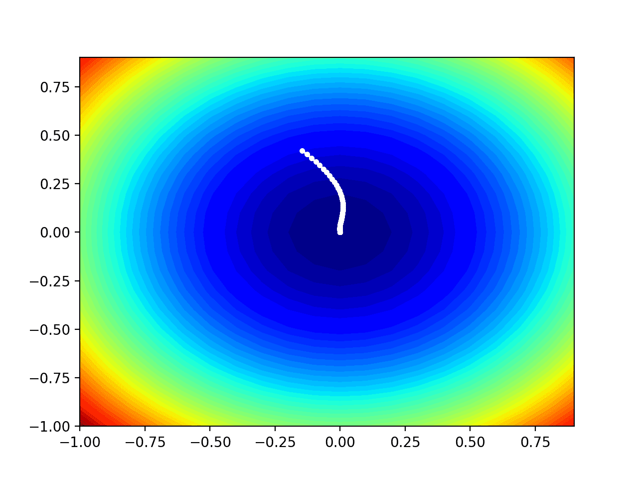
Contour Plot of the Test Objective Function With AdaMax Search Results Shown
Further Reading
This section provides more resources on the topic if you are looking to go deeper.
Papers
- Adam: A Method for Stochastic Optimization, 2014.
- An Overview Of Gradient Descent Optimization Algorithms, 2016.
Books
- Algorithms for Optimization, 2019.
- Deep Learning, 2016.
APIs
Articles
- Gradient descent, Wikipedia.
- Stochastic gradient descent, Wikipedia.
- An overview of gradient descent optimization algorithms, 2016.
Summary
In this tutorial, you discovered how to develop the gradient descent optimization with AdaMax from scratch.
Specifically, you learned:
- Gradient descent is an optimization algorithm that uses the gradient of the objective function to navigate the search space.
- AdaMax is an extension of the Adam version of gradient descent designed to accelerate the optimization process.
- How to implement the AdaMax optimization algorithm from scratch and apply it to an objective function and evaluate the results.
Do you have any questions?
Ask your questions in the comments below and I will do my best to answer.
The post Gradient Descent Optimization With AdaMax From Scratch appeared first on Machine Learning Mastery.