Multiple linear regression with Python, numpy, matplotlib, plot in 3d

[Charles Durfee]

Background info / Notes:

Equation:
Multiple regression: Y = b0 + b1*X1 + b2*X2 + … +bnXn
compare to Simple regression: Y = b0 + b1*X

In English:
Y is the predicted value of the dependent variable
X1 through Xn are n distinct independent variables
b0 is the value of Y when all of the independent variables (X1 through Xn) are equal to zero
b1 through bn are the slope of the relationship between the dependent variable and the independed variable that is holding constant of all other independent variables.

Think of it as a system of equations:
Y1 = (b + mX1) + e1
Y2 = (b + mX2) + e2
…
Yn = (b + mXn) + en
We can then set up a matrix equation with the following matrices:

     |Y1|
Y =  |...|
     |Yn|

     |1 X1|
X =  |...|
     |1 Xn|

    |b|
A = |m|

    |e1|
E = |...|
    |en|

Which gives us the matrix equation: Y = XA + E
We just need to solve for A

Use Linear Algebra to solve
Equation:
A = (X^T * X)^-1 * (X^T * Y)

Two helpful links that explain how we get this equation:
https://www.youtube.com/watch?v=Qa_FI92_qo8
https://www.youtube.com/watch?v=qdOG7YMolmA

Convert the equation to code:
Using the np.linalg.solve function we will not need to invert the first term
a = np.linalg.solve(np.dot(X.T, X), np.dot(X.T, Y))

You can download the code or dataset from github here.

The full code:

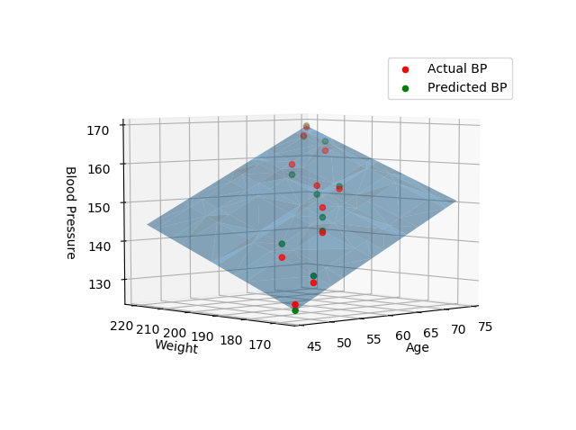
import numpy as np
import matplotlib.pyplot as plt
from mpl_toolkits.mplot3d import Axes3D

# create arrays for the data points
X = []
Y = []

#read the csv file
csvReader = open('BloodPressure.csv')

#skips the header line
csvReader.readline()

for line in csvReader:
    y, x1, x2 = line.split(',')
    X.append([float(x1), float(x2), 1]) # add the bias term at the end
    Y.append(float(y))

# use numpy arrays so that we can use linear algebra later
X = np.array(X)
Y = np.array(Y)

# graph the data
fig = plt.figure(1)
ax = fig.add_subplot(111, projection='3d')
ax.scatter(X[:, 0], X[:, 1], Y)
ax.set_xlabel('Age')
ax.set_ylabel('Weight')
ax.set_zlabel('Blood Pressure')

# Use Linear Algebra to solve
a = np.linalg.solve(np.dot(X.T, X), np.dot(X.T, Y))
predictedY = np.dot(X, a)

# calculate the r-squared
SSres = Y - predictedY
SStot = Y - Y.mean()
rSquared = 1 - (SSres.dot(SSres) / SStot.dot(SStot))
print("the r-squared is: ", rSquared)
print("the coefficient (value of a) for age, weight, constant is: ", a)

# create a wiremesh for the plane that the predicted values will lie
xx, yy, zz = np.meshgrid(X[:, 0], X[:, 1], X[:, 2])
combinedArrays = np.vstack((xx.flatten(), yy.flatten(), zz.flatten())).T
Z = combinedArrays.dot(a)

# graph the original data, predicted data, and wiremesh plane
fig = plt.figure(2)
ax = fig.add_subplot(111, projection='3d')
ax.scatter(X[:, 0], X[:, 1], Y, color='r', label='Actual BP')
ax.scatter(X[:, 0], X[:, 1], predictedY, color='g', label='Predicted BP')
ax.plot_trisurf(combinedArrays[:, 0], combinedArrays[:, 1], Z, alpha=0.5)
ax.set_xlabel('Age')
ax.set_ylabel('Weight')
ax.set_zlabel('Blood Pressure')
ax.legend()
plt.show()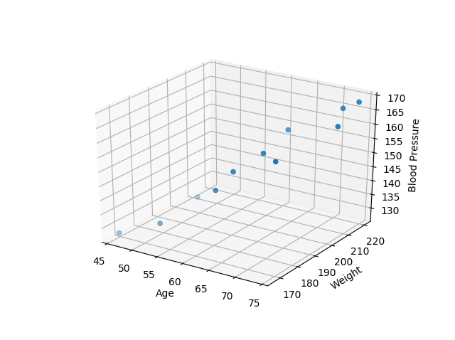

[Author]

Posts